Accelerated MVA in triCalculate

The phased introduction of bilateral initial margin is affecting institutions with gradually decreasing size. Institutions that stand to benefit the most from a central analytics service are coming into scope and, as a response, triCalculate has added margin valuation adjustment (MVA) to the catalogue of risk metrics. 

 

Consistent global modelling

Traditional XVA systems separate the tasks of generating market factor paths and pricing netting set values. Paths for each market factor are generated using a simulation model, which is calibrated to traded instruments. The netting set value for each path and time step is obtained by feeding the simulated market state into separate independent pricing models. The pricing models generally imply a different dynamic behaviour of the underlying to the dynamics assumed by the simulation model in the path generation phase. This mismatch ultimately leads to XVA inaccuracies as well as mismatching hedging strategies. 

The Probability Matrix Method – as introduced by Albanese et al – is more consistent. The modelling framework is based on common transition probability matrices for generating scenarios and pricing netting sets. Provided with calibrated models, the first step is to generate transition probability matrices on a predefined discrete time-and-space grid. The second step involves using the generated matrices to price all derivatives contracts to obtain valuation tables expressing the value of every netting set in every discrete state of the world. The transition probability matrices are again used in the third step to generate simulation paths for the underlying market factors. Market factors are correlated using a Gaussian copula, which is typically calibrated to historical time series. Finally, in the fourth step, XVA is calculated by stepping through simulation paths, looking up the netting set values in the valuation tables and evaluating the XVA contributions. 

The clear separation of computation tasks into the steps described above has proven to be extremely effective – from the point of view of performance as well as development. Pre-computing transition probability matrices and valuation tables, using graphics processing unit (GPU) technology, allows for a simplified simulation procedure that significantly cuts overall computation time by orders of magnitude. This raw power facilitates a simple and uncompromising implementation of MVA. Where many authors advocate approximations for evaluating the initial margin formula, the sheer speed of the triCalculate engine allows for full valuation in every time step, along every path.

 

MVA calculation

The standard credit valuation adjustment (CVA) and funding valuation adjustment (FVA) calculations are trivial exercises once we have generated scenarios and valuation tables as described above. In every step along the path, we simply need to look up the netting set value from a table rather than firing up an external pricing engine. MVA presents a further challenge, however. As in Green and Kenyon, we define MVA as an expectation of an integral according to:  

where st is the funding spread over the initial margin collateral rate, λC s and
λB s are the (dynamic) default intensities of the counterparty and the bank respectively, and Mt is the initial margin amount.

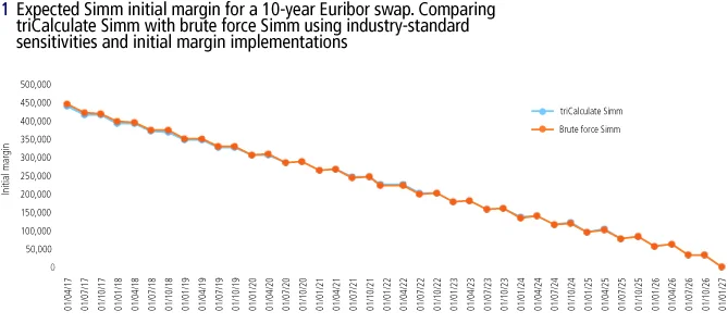
This expression is very similar to the expressions for the traditional XVA measures CVA and FVA. The complicating factor is that the initial margin is a rather complex quantity to calculate along the path. The standard initial margin model (Simm) bilateral initial margin formula takes bucketed netting set sensitivities as input, and value-at-risk or expected shortfall-based clearing house initial margin can be simplified using delta/gamma type expansions also requiring bucketed netting set sensitivities to be calculated (see figure 1).  

Fortunately, the valuation table generation in the Probability Matrix Method responds very well to bucketed netting set sensitivity calculations. Experience has shown that clever chain-rule applications – or adjoint algorimithic differentiation – is only needed for the simulation step when calculating regular XVA sensitivities. For MVA we may rely on standard perturbation techniques to generate the bucketed netting set sensitivities we need. The reason netting set sensitivity calculation scales so well with the number of sensitivities is down to the use of GPU hardware. The operation of transferring memory to the GPU device is the bottleneck that constrains GPU performance. This means there is often spare capacity to be used on the GPU while memory is being copied back and forth during execution. Sensitivity calculations are efficiently utilising this spare capacity as more computations can be performed on each batch of data. 

For the MVA calculation we generate not only the valuation tables containing netting set values during the valuation step, but also tables containing the bucketed netting set sensitivities for every future state of the world. Despite the minor complexity of the Simm formula, the simulation step is still a simple exercise of simulating the market factors forward, looking up the bucketed netting set sensitivities and evaluating the initial margin formula. 

 

Test results and performance 

To benchmark the MVA calculation we turn to two initial margin-related services actively used by the industry today: The Acadia IM Exposure Manager, powered by TriOptima, and the triBalance initial margin optimisation service. First, we generate and export 1,000 paths with quarterly time steps from triCalculate. Simm sensitivities are generated for every path and every time step using the infrastructure and models used to generate triBalance initial margin optimisation proposals. The sensitivities are then fed to the IM Exposure Manager Simm implementation, which produces an initial margin number for every simulation date in every path. 

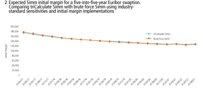
The end-result of this exercise is essentially a brute force MVA calculator, which we use to benchmark the triCalculate expected initial margin curves. Results can be observed in figures 1 and 2, where we compare the expected Simm initial margin for a standalone swap and a standalone swaption, respectively. 

3 Calculation time

Example of calculation time when running MVA on a diversified portfolio on a standard laptop computer using the Probability Matrix Method

• 100,000 paths
• Quarterly time steps
• 50 counterparties
• 20,000 trades
• Intel i7 2.6GHz
• 8GB RAM
• NVIDIA GTX 950M
• Valuation: 132 seconds
• Simulation: 65 seconds
• Total time: 197 seconds

The naive brute force MVA implementation takes hours to run while the triCalculate initial margin profile is generated in minutes. To further highlight the performance of the Probability Matrix Method, figure 3 provides an example of calculation times when calculating MVA on a realistic portfolio using a standard laptop computer.

Sponsored content