Hedging of financial derivative contracts via Monte Carlo tree search

Oleg Szehr

Abstract

The construction of replication strategies for the pricing and hedging of derivative contracts in incomplete markets is a key problem in financial engineering. We interpret this problem as a “game with the world”, where one player (the investor) bets on what will happen and the other player (the market) decides what will happen. Inspired by the success of the Monte Carlo tree search (MCTS) in a variety of games and stochastic multiperiod planning problems, we introduce this algorithm as a method for replication in the presence of risk and market friction. Unlike model-free reinforcement learning methods (such as Q-learning), MCTS makes explicit use of an environment model. The role of this model is taken by a market simulator, which is frequently adopted even in the training of model-free methods, but its use allows MCTS to plan for the consequences of decisions prior to the execution of actions. We conduct experiments with the AlphaZero variant of MCTS on toy examples of simple market models and derivatives with simple payoff structures. We show that MCTS is capable of maximizing the utility of the investor’s terminal wealth in a setting where no external pricing information is available and rewards are granted only as a result of contractual cashflows. In this setting, we observe that MCTS has superior performance compared with the deep Q-network algorithm and comparable performance to “deep-hedging” methods.

Download PDF

Introduction

1 Introduction

Monte Carlo tree search (MCTS) is a class of model-based reinforcement learning (RL) algorithms for the approximation of optimal decisions in multiperiod planning problems under uncertainty. At its core, MCTS maintains a problem-specific decision tree, where states are evaluated by averaging over Monte Carlo trajectories of plausible courses of action and model behavior. A domain generative model provides samples of state–action–state transitions for the construction of the decision tree, and a dedicated tree policy guides the construction to relevant courses of action. In artificial intelligence (AI), MCTS-type algorithms constitute the state of the art and the most well-researched method for a wide range of planning problems, with discrete perfect information scenarios (in certain games and puzzles) at the one end and continuous imperfect information scenarios (in real-world decision-making) at the other. Typical examples of application include combinatorial puzzles (in a one-player setting), combinatorial games (chess and go, in a two-player setting) and problems from combinatorial optimization (the traveling salesman problem), but also nondeterministic and imperfect information domains (poker or the sailing domain) and domains with continuous state and action spaces (as in robotics or games such as StarCraft) (see Browne et al (2012) and Świechowski et al (2022) for reviews of applications and the state of the art). This paper introduces the application of MCTS to an important stochastic planning problem in finance: the pricing and hedging of financial derivatives contracts.

The modern derivatives pricing theory came to light with two papers, by Black and Scholes (1973) and Merton (1973), on the valuation of European option contracts. They introduce what is now known as the Black–Scholes–Merton (BSM) economy: a model of a financial market comprised of a risk-free asset (called a “bond” or “cash”), a risky asset (the “stock”) and an asset whose price is contingent on the behavior of the risky asset (thus, a “derivative”). The risk-free asset exhibits a constant rate of interest, while the risky asset promises higher returns but bears market fluctuations following a continuous-time geometric Brownian motion (GBM) process. The derivative, a European call option, gives its holder the right to buy shares of a stock at an agreed price on an agreed future date. Black and Scholes (1973) and Merton (1973) show that in their economy there exists a self-financing, continuous-time trading strategy in the risk-free asset and the stock that exactly replicates the value (ie, price) of the option contract over the investment horizon. Thus, a negative replicating portfolio can be maintained to offset (“hedge”) the risk involved in the option contract. The absence of arbitrage then dictates that the option price must be equal to the cost of setting up the replicating portfolio. In reality, continuous-time trading is of course impossible. It cannot even serve as an approximation due to the resulting high transaction costs. In other words, transaction costs create market incompleteness: the derivative contract cannot be hedged exactly and, as a consequence, its issuer incurs risk. Since hedging under market incompleteness involves risky positions, it follows that the price depends on the risk preference of the investor. Hence, in reality, the hedging problem is “subjective” – it depends on the investor’s utility.

In more modern terms, the replication and pricing problems are often formulated as stochastic multiperiod utility optimization problems (Duffie 2001): in order to hedge a derivative contract, an economic agent consecutively buys/sells shares of stock so as to maximize the expected utility of their terminal holdings. Although the specific setup varies, many such problems can be phrased in the language of dynamic programming with an accompanying Bellman equation. This makes dynamic programming and RL natural and well-studied tools for hedging and pricing (see, for example, Hodges and Neuberger (1989), Barron and Jensen (1990), Karoui and Quenez (1995), Zakamouline (2006) and the references therein). More recently, RL gained wide public attention when agents using a combination of RL and neural network (NN) techniques reached superhuman levels of play in a variety of games, including Atari games (Mnih et al 2013), go (Silver et al 2017) and chess (Silver et al 2018). This advancement has also reached the field of financial derivatives, where several publications reported on the promising performance of “deep” RL agents (see, for example, Halperin 2017; Kolm and Ritter 2019; Cao et al 2021; Bisi et al 2020; Vittori et al 2020). In terms of the choice of algorithm, an important role is played by variations of $Q$-learning (Watkins and Dayan 1992), specifically by the deep $Q$-network (DQN) algorithm of Mnih et al (2013), which employs an NN for the representation of state–action values (see, for example, Halperin 2017; Kolm and Ritter 2019; Cao et al 2021). Being a model-free RL algorithm, $Q$-learning learns solely from the rewards it observes in operation. Thus, the DQN algorithm could, in principle, learn from the real markets without an auxiliary model environment being set up. In reality, however, the amount of data required for training a DQN hedger is significantly larger than that available from derivatives markets. This is demonstrated by the data requirement reported by Kolm and Ritter (2019) and Cannelli et al (2023) and the fact that Halperin (2017), Kolm and Ritter (2019), Cannelli et al (2023) and Cao et al (2021) all assume an accurate market simulator (see also our experiments below). In this sense it can hardly be claimed that the trained agents operate in a fully model-free setup. Model-based RL and supervised learning thus offer themselves as natural alternatives.

In contrast to model-free methods (such as $Q$-learning), model-based RL (such as MCTS) leverages an environment/domain model to predict the consequences of possible courses of action in terms of future states and rewards. This allows for RL architectures that plan their decisions in view of the exploration and exploitation of rewards prior to executing actions. For example, in the case of MCTS a problem-specific Monte Carlo planning tree is constructed to estimate $Q$-values, in contrast to plain Monte Carlo temporal-difference updates of $Q$-values in $Q$-learning. The MCTS is designed to approximate the optimal policies for multiperiod planning problems within the framework of Markov decision processes (MDPs). Prototypical MCTS variants, such as upper confidence bounds applied to trees (UCT) (Kocsis and Szepesvári 2006) or maximum entropy for tree search (MENTS) (Xiao et al 2019), converge to optimal policies for general MDPs in the sense that the probability of taking suboptimal actions goes to zero in the limit of large resources (see Kocsis and Szepesvári 2006; Xiao et al 2019).

It should come as no surprise that for many planning problems, planning-based methods learn stronger policies faster and achieve higher performance scores than the best model-free approaches. For example, MCTS variants outperform model-free methods in numerous video games.¹¹ 1 See the performance of MCTS agents in the planning track (Torrado et al 2018) of the General Video Game AI competition (Pérez-Liébana et al 2019) and the Arcade Learning Environments (Atari games) (Guo et al 2014). These variants also commonly outperform model-free methods in terms of their generalization capability, ie, their ability to operate in previously unseen scenarios (given some high-level description of the task, such as the rules of a game). An example is MCTS’s effectiveness in general game playing (see, for example, Finnsson and Björnsson 2008), where “almost every general game playing program today uses some version of MCTS” (Genesereth and Björnsson 2013). The MCTS underlies the AlphaZero algorithm and its tremendous success in strategy games such as hex (Anthony et al 2017), go (Silver et al 2017) and chess (Silver et al 2018), in which it achieves higher performance scores than supervised learning and model-free RL. The application of MCTS to stochastic multiperiod planning is apparent in its roots, where, for example, the sailing domain (Vanderbei 1996) served as a popular test bed for early MCTS variants (Péret and Garçia 2004; Kocsis and Szepesvári 2006).²² 2 The sailing domain is a finite-state-and-action-space, discrete-time, stochastic shortest-path problem, where a sailboat searches for the shortest path between two points of a grid under fluctuating wind conditions. The sailing domain and the recent application of MCTS to planning problems in energy markets (Couëtoux 2013) display considerable similarities with derivatives hedging, and it a popular interpretation of derivatives pricing and hedging is “a game with the world” (Shafer and Vovk 2001). In this game, one player (the investor) bets on what will happen and the other player (the market) decides what will happen. Shafer and Vovk (2001) demonstrate that this interpretation is fundamental, and it may take an axiomatic role in the construction of financial mathematics and probability theory in general. The application of tree-search techniques in the field of derivatives is equally unsurprising. Tree models have served as discrete approximation methods for the valuation of derivative contracts for decades (Cox et al 1979; Boyle 1986) and were employed as a tool for utility optimization and the computation of reservation price in the pioneering work of Hodges and Neuberger (1989). The main idea behind the application of MCTS might be seen in learning tree-based approximations efficiently. The MCTS achieves this by problem-specific Monte Carlo sampling with an emphasis on relevant market moves and actions.

Several alternatives to planning-based derivatives hedging should be mentioned. First, there is an extensive classical literature on stochastic optimal control, dynamic programming, etc (see above). Second, there is the “semisupervised” setting of Kolm and Ritter (2019), Vittori et al (2020) and Bisi et al (2020). In this setting, derivative prices are known a priori (eg, through a pricing engine) and RL is typically employed to trade off transaction costs against replication errors. This is studied by Kolm and Ritter (2019) using a risk-averse DQN algorithm and by Vittori et al (2020) using a risk-averse policy search (Bisi et al 2020). Third, Halperin (2017) and Cao et al (2021) employ the DQN without external price information, but they simplify the learning process by setting up a mathematical methodology that translates contractual cashflows into reward portions awarded after individual hedging decisions. Another line of research entirely gives up multiperiod planning for derivatives hedging (Cannelli et al 2023). This is motivated by the high data requirement of full-fledged RL and the practical operations of investment firms that often require the end-of-day reporting of risk figures. Finally, an important alternative to RL is provided by the “deep-hedging” approach of Buehler et al (2019a, b), who approach utility optimization as a recursive supervised learning exercise.³³ 3 There is also an interpretation of this work in the context of RL (Buehler et al 2019b). We prefer to view it as supervised learning due to the absence of explicit exploration in “deep-hedging” policies. In this approach, an NN-based optimization is carried out simultaneously over the whole sequence of hedging decisions and the price of setting up the replication portfolio. In sophisticated domains such as chess or go, straightforward gradient descent optimization can easily get stuck at a poor local optimum because of the high complexity of the value function or a nondifferentiable reward structure. However, in common hedging scenarios a stable and sample-efficient approach to the hedging problem is provided by gradient-descent-based optimization, which also scales favorably in multiasset portfolio optimization tasks (Buehler et al 2019a).

In the practical work of an investment firm, the availability of real-world data for training will often constitute a bottleneck for the deployment of any form of AI for hedging. The generalization capability of AI systems might point to a potential way out in that a system could be pretrained on simulated data and then executed and fine-tuned on available real-world data. Unlike supervised learning, MCTS is also capable of generating the samples it requires for training through adversarial self-play. It is conceivable that MCTS could be pretrained on a list of preselected models of markets, costs, etc, or in a model-free agent-versus-market setup similar to that of Silver et al (2017), although this remains a topic for future research. In summary, the following points motivate our investigation of MCTS in the context of financial derivatives contracts.

1. (1)

   The MCTS approaches pricing and hedging directly, through the maximization of the utility of terminal wealth in the respective multiperiod optimal control problems. Rewards are only granted as a consequence of contractual cashflows. No intermediate reward signals and no external pricing information are required.

2. (2)

   The MCTS is a model-based planning algorithm. It makes explicit use of given models of markets, transaction costs, utility, price, etc, to plan for and optimize the outcomes of actions prior to their execution. Model-free methods optimize decisions based solely on historic reward information.

3. (3)

   MCTS variants constitute the state of the art in a variety of specific games and in general game playing. We expect a competitive performance from MCTS in the comparatively simple pricing and hedging games.

4. (4)

   MCTS variants possess convergence guarantees in a general MDP context, converging to optimal actions if sufficient resources are granted. The MCTS is thus applicable for wide classes of Markovian models of markets, transaction costs, utility, price, etc.

In this paper we conduct experiments using the AlphaZero algorithm (Silver et al 2017), which combines MCTS with NNs, on toy examples of market models and derivative contracts with simple payoff structures. In particular, we test our AlphaZero variant on discrete (trinomial) and discretized versions of continuous (GBM, Heston) market models with and without transaction costs. Our interest in the AlphaZero variant is motivated by

1. (1)

   the flexibility of NNs as universal function approximators;

2. (2)

   AlphaZero’s ability to operate in large state and action spaces, which we expect to occur through discretization of continuous market models; and

3. (3)

   a potential application of our architecture in larger-scale systems, where the coordination of buys and sells requires intelligent behavior (eg, in view of system scalability and book-dependent asset pricing).

In our experiments we compare AlphaZero with the DQN in a setting where rewards are only generated as a result of contractual cashflows. In this setting the DQN’s performance turns out to be poor. We proceed by simple benchmark experiments of AlphaZero against “deep-hedging” with a feedforward NN (FF-NN). We observe an overall comparable performance, but seemingly a slightly greater sample efficiency for AlphaZero. Finally, it should be mentioned that MCTS also has several disadvantages. Compared with supervised learning and the DQN, MCTS is more complex and more difficult to maintain and its results are harder to interpret. Training and execution are typically much slower in MCTS. The choice of reward function and model calibration took considerable effort in our experiments.

2 The hedging and pricing problems

We consider an economy composed of cash, shares of a risky asset and a derivative contract. Let $S_t$ denote the price of the risky asset at time $t$ and let $B_t$ denote the bank account holdings of an investor.⁴⁴ 4 For simpler notation we assume that there is no interest on cash. We assume a Markovian market and that new market information becomes available at discrete times $t=1,2,\mathrm{\dots },T$. At time $t=0$ the investor sells the derivative with underlying $S_t$. As a result, an immediate profit $B_0\ge 0$ is credited to the investor’s bank account, but the derivative also creates a random liability of  at contract maturity $T$. In order to offset the risk from this liability, the investor maintains a hedging portfolio of the form

$${\mathrm{\Pi }}_t=n_t{S}_t+B_t$$

with $n_t$ shares of the risky asset. The investor’s wealth $w_t$ is then composed of the replication portfolio ${\mathrm{\Pi }}_t$ and the negative price, $Z_t$, of the derivative contract. Shortly before new market information becomes available, the investor decides upon a new portfolio composition. Formally, the agent’s objective is to choose a trading strategy (policy, see below) to maximize the expected utility,

$\underset{n_1,\mathrm{\dots },n_T}{\max }𝔼[u(w_T)],$

(2.1)

of terminal wealth subject to additional capital constraints. The utility function $u$ quantifies the investor’s risk preference and is usually smooth and strictly increasing. Capital constraints ensure the problem remains self-contained in the sense that trading strategies will neither require nor generate external funds by themselves. Note that in (2.1) the sell price $B_0$ is given exogenously; that is, it applies in a situation where the contract has already been sold. Pricing is discussed below. We refer the reader to Duffie (2001) for a detailed introduction to dynamic asset allocation.

2.1 The complete market

The complete market is characterized by the assumption that all derivatives can be replicated exactly. Replication strategies must be self-financing; that is, any purchase/sale of shares is reflected by a respective transaction on the bank account. If at time $t$ a number $\mathrm{\Delta }{n}_{t+1}$ of shares is bought/sold at price $S_t$, then in the absence of transaction costs this is reflected in the bank account by a debit/credit of $\mathrm{\Delta }{B}_{t+1}=-\mathrm{\Delta }{n}_{t+1}{S}_t$.⁵⁵ 5 We use the notation $\mathrm{\Delta }{X}_{t+1}=X_{t+1}-X_t$ throughout the paper. The corresponding change in the replication portfolio is

$$\mathrm{\Delta }{\mathrm{\Pi }}_{t+1}=n_{t+1}\mathrm{\Delta }{S}_{t+1}.$$

When starting with an initial value of ${\mathrm{\Pi }}_0$ (from the sell price of the derivative), this implies

$${\mathrm{\Pi }}_T={\mathrm{\Pi }}_0+\sum _{t=0}^{T-1}{n}_{t+1}\mathrm{\Delta }{S}_{t+1}.$$

The dynamic-programming view on the hedging problem is as follows: at contract maturity the investor’s terminal wealth is the sum of the terminal investment portfolio, ${\mathrm{\Pi }}_T$, and the contractual liability, $Z_T$. One time step before maturity the agent holds a replication portfolio ${\mathrm{\Pi }}_{T-1}$ consisting of $B_{T-1}$ units of cash and $n_{T-1}$ shares of the risky asset at price $S_{T-1}$. The agent adjusts the number of shares $n_T$ for the subsequent period so as to maximize the conditional expected utility of the terminal holdings:

$$𝔼[u({\mathrm{\Pi }}_T+Z_T)\mid {ℱ}_{T-1}]=𝔼[u({\mathrm{\Pi }}_{T-1}+n_T\mathrm{\Delta }{S}_T+Z_T)\mid {ℱ}_{T-1}].$$

Conditioning on the filtration ${ℱ}_t$ means that all market information at time $t$, including $S_t$, ${\mathrm{\Pi }}_t,\mathrm{\dots },$ is realized and available for decision-making. The agent proceeds by planning backward in time. Two steps before maturity the agent adjusts $n_{T-1}$ to maximize the above expectation conditioned on ${ℱ}_{T-2}$, three steps before maturity the agent chooses $n_{T-2}$ conditioned on ${ℱ}_{T-3}$, and so on. The optimal course of action corresponds to the optimal value function:

$$V^{*}(t,S_t,{\mathrm{\Pi }}_t):=\underset{n_1,\mathrm{\dots },n_T}{\max }𝔼[u({\mathrm{\Pi }}_T+Z_T)\mid {ℱ}_t].$$

As described in Section 2.4, $V^{*}$ will be a solution of a Bellman optimality equation.

In a complete market, the possibility of perfectly offsetting any derivative contract implies an “automatic” pricing mechanism via the no-arbitrage principle (Delbaen and Schachermayer 2006): the fair price is simply the cost of setting up the replication portfolio. When no perfect replication is possible, pricing becomes nonunique.

Example 2.1 (BSM hedges (Merton 1990)).

BSM pricing and hedging rely on the paradigm that the replication portfolio should exactly offset the derivative contract at all times. Accordingly, at each step of the backward planning process the investor chooses the portfolio composition so as to minimize the risk of the consecutive period. Suppose $S_t$ is of GBM type and the investor hedges a European vanilla call option with the payoff $Z_T(S_T)=C_T(S_T)=-{(S_T-K)}^{+}$. Let the investor’s terminal wealth be split into an initial wealth amount and a series of increments $w_T=w_0+{\sum }_t\mathrm{\Delta }{w}_{t+1}$. Suppose the agent maximizes (2.1) by minimizing the risk of individual wealth increments of the form

$${\text{Risk}}_t=𝔼[{(\mathrm{\Delta }{w}_{t+1})}^2\mid {ℱ}_t].$$

This corresponds to a utility that is additive with respect to the individual wealth increments $u(w_T)={\sum }_t{u}_t(\mathrm{\Delta }{w}_{t+1})$ with quadratic $u_t$. At each time step the price $C_t$ can be defined as the minimizer of ${\text{Risk}}_t$ given the optimal hedge. In the limit of continuous time and continuous hedges, this leads to the $\delta$-hedge portfolio, $n_{t+1}\to {\delta }_t=\partial C_t^{*}/\partial S_t$, where $C_t^{*}$ is the BSM option price. In this case the global utility minimum is reached; by following the $\delta$-hedging strategy, the agent does not take any risk, and any deviation from this strategy results in a risky position.

2.2 Incomplete markets and pricing

Common reasons for market incompleteness include transaction costs, the presence of stochastic volatility (Hull and White 1987) and jump-diffusion price processes (Aase 1988). In the presence of transaction costs the self-financing constraint must be adjusted, where each trading activity is accompanied by a loss of . In other words,

${\mathrm{\Pi }}_{t+1}-{\mathrm{\Pi }}_t=n_{t+1}\mathrm{\Delta }{S}_{t+1}+\mathrm{cost}(n_t,n_{t+1},S_t).$

(2.2)

The dynamic programming approach remains valid, but the structure of the hedging problem might require additional state variables. For example, proportional transaction costs $\mathrm{cost}(n_t,n_{t+1},S_t)=-\eta |\mathrm{\Delta }{n}_{t+1}|S_t$ depend on the current holdings $n_t$, whereas the BSM’s $\delta$-hedges do not. In a similar vein, additional state variables emerge in the presence of stochastic volatility and interest rates. Various models have been proposed to address pricing and hedging in incomplete markets. One prominent line initiated by Föllmer and Sondermann (1986) (see also Bouchaud and Sornette 1994; Schäl 1994; Schweizer 1995) considers pricing through a risk-minimization procedure. The “fair hedging price” (Schäl 1994) of a derivative with liability $Z_T$ is the minimizer of the risk

$${\mathrm{\Pi }}_0^{*}=\underset{{\mathrm{\Pi }}_0}{\arg \min }\left[\underset{n_1,\mathrm{\dots },n_T}{\min }𝔼[-u({\mathrm{\Pi }}_T+Z_T)]\right].$$

We illustrate this by a standard example (see, for example, Föllmer and Sondermann 1986; Schweizer 1995).

Example 2.2.

(Terminal variance hedging)  The problem is to minimize the expected net quadratic loss

$$\underset{{\mathrm{\Pi }}_0,n_1,\mathrm{\dots },n_T}{\min }𝔼[{({\mathrm{\Pi }}_T+Z_T)}^2]$$

simultaneously over the initial cash balance ${\mathrm{\Pi }}_0$ and the decisions $n_1,\mathrm{\dots },n_T$. Dynamic programming applies to this problem, where the value function involves an additional optimization over ${\mathrm{\Pi }}_0$,

$$V^{*}(t,S_t,{\mathrm{\Pi }}_t)=\underset{{\mathrm{\Pi }}_0,n_1,\mathrm{\dots },n_T}{\min }𝔼[{({\mathrm{\Pi }}_T+Z_T)}^2\mid {ℱ}_t].$$

Assuming no transaction costs and sufficient regularity for $S_t$, the optimal price and hedges can be computed explicitly (Schweizer 1995). If the price ${\mathrm{\Pi }}_0^{*}$ and the investment decisions $n_1({\mathrm{\Pi }}_0^{*}),\mathrm{\dots },n_T({\mathrm{\Pi }}_0^{*})$ solve the optimization problem, then these decisions are also optimal for the minimization of the terminal variance (TV) ${\min }_{n_1,\mathrm{\dots },n_T}𝕍[{\mathrm{\Pi }}_T+Z_T]$.

This form of pricing ignores the possibility that a portfolio without liabilities could have a positive value. The main idea behind the concept of reservation price (Hodges and Neuberger 1989; Davis et al 1993; Clewlow and Hodges 1997; Zakamouline 2006) is that buy/sell prices of derivative contracts should be such that the buyer/seller remains indifferent, in terms of expected utility, with respect to the following two situations:

1. (1)

   purchasing/selling a number of derivative contracts and hedging the resulting risk by a portfolio of existing assets, or

2. (2)

   leaving the wealth optimally invested within existing assets and not entering new contracts.

Suppose an investor sells a derivative at time $t$ and is not allowed to trade it thereafter. The seller’s problem is to maximize the expected utility,

$$V_{\text{sell}}^{*}(t,n_t,S_t,{\mathrm{\Pi }}_t)=\max 𝔼[u({\mathrm{\Pi }}_T+Z_T)\mid {ℱ}_t],$$

subject to (2.2). In the absence of derivative contracts, the investor simply optimizes

$${\tilde{V}}^{*}(t,n_t,S_t,{\mathrm{\Pi }}_t)=\max 𝔼[u({\mathrm{\Pi }}_T)\mid {ℱ}_t].$$

The reservation sell price of a derivative with liability $Z_T$ is defined as the price $P^s$ such that

$${\tilde{V}}^{*}(t,n_t,S_t,{\mathrm{\Pi }}_t)=V_{\text{sell}}^{*}(t,n_t,S_t,{\mathrm{\Pi }}_t+P^s).$$

The definition of the buy price is analogous. In the BSM economy, buy and sell reservation prices converge to the familiar BSM pricing formulas. The computation of the reservation price under general assumptions is often a difficult problem. An important special case occurs when the investor’s utility function exhibits a constant absolute risk aversion (CARA) and transaction costs are proportional to the traded volume of underlying shares. Notably, the reservation prices of the CARA investor can also be viewed as risk-minimization prices with respect to an entropic risk measure (Buehler et al 2019a). Next we give an example of Hodges–Neuberger (HN) exponential utility hedges (Hodges and Neuberger 1989; Davis et al 1993).

Example 2.3 (HN exponential utility hedges).

Assuming a constant proportional cost model, $\mathrm{cost}(n_t,n_{t+1},S_t)=-\eta |\mathrm{\Delta }{n}_{t+1}|S_t,$ and an exponential utility of terminal wealth with CARA,

$$u(w_T)=-\exp (-\lambda w_T),$$

results in trading strategies that are wealth independent and that do not create risky positions when no derivative contract is traded. The portfolio allocation space is divided into three regions: the buy region, the sell region and the no-transaction region. If the portfolio lies in the buy/sell region, then the optimal strategy is to buy/sell shares of the risky asset until the portfolio reaches the boundary between the buy/sell region and the no-transaction region. If a portfolio is located in the no-transaction region, then it is not adjusted at that time step.

2.3 MDPs and RL

MDPs are a mathematical framework for sequential decision problems in uncertain dynamic environments (Sutton and Barto 2018). Formally, an MDP is a five-tuple $(S,A,P,R,T)$ with a set of admissible states $S=\{s^{(1)},\mathrm{\dots },s^{(n)}\}$, a set of possible actions $A=\{a^{(1)},\mathrm{\dots },a^{(m)}\}$, a transition probability function $P:S\times A\times S\to [0,1]$ defining the probability $P(s^{\prime }\mid a,s)$ of entering state $s^{\prime }$ by taking action $a$ in state $s$, and a reward $R(s,a)$ granted through this transition.⁶⁶ 6 We assume that $S$ and $A$ are finite in our explanations, but in some of our experiments an infinite state space will occur. In MDPs an agent interacts iteratively with an environment over a sequence of time steps $t=0,1,2,\mathrm{\dots },T-1$. In each step the agent observes the current state $s_t$ and takes a respective action $a_t$ according to a policy $\pi (a_t\mid s_t)$; then, the environment transitions to $s_{t+1}$ according to $P(s^{\prime }=s_{t+1}\mid a=a_t,s=s_t)$ and a reward of $R_t(s_t,a_t)$ is granted to the agent. The agent considers the new state $s_{t+1}$, takes a respective action and the environment transitions to the subsequent state for a total of $T$ iterations. The value function associates with each state $s$ the expected total reward when starting at $s$ and following $\pi$:

$$V^{\pi }(s)={𝔼}_{\pi }\left[\sum _{t=0}^{T-1}{\gamma }^t{R}_t(s_t,a_t)\right|s_0=s].$$

The role of the factor $\gamma \in [0,1]$ is to quantify the relevance, in terms of total reward, of the immediate consequences of an action versus its long-term effect. Similarly, the action value function (also known as the quality function) $Q^{\pi }(s,a)$ is defined as the expected total reward when starting from $s$, taking the action $a$ and thereafter following $\pi$:

$Q^{\pi }(s,a)={𝔼}_{\pi }\left[{\displaystyle \sum _{t=0}^{T-1}}{\gamma }^t{R}_t(s_t,a_t)\right|s_0=s,a_0=a].$

(2.3)

The agent’s goal is to find a policy that maximizes the expected total reward. It is a classical result that the optimal value function

$$V^{*}(s)=V^{{\pi }^{*}}(s)=\underset{\pi }{sup}{V}^{\pi }(s)$$

satisfies the Bellman optimality equation

$V_t^{*}(s)=\underset{a}{\max }\left\{R_t(s,a)+\gamma {\displaystyle \sum _{s^{\prime }\in S}}P(s^{\prime }\mid s,a)V_{t+1}^{*}(s^{\prime })\right\}.$

(2.4)

RL is an iterative process in which an agent learns to accumulate rewards in an MDP setting. The learning process is commonly organized into a number of independent training episodes, each corresponding to the full execution of the agent’s MDP task, such as playing a game from beginning to end or hedging a derivative from inception to maturity. By executing episodes repeatedly, the agent learns to maximize the expected accumulated rewards by adapting their policy. A key point is that in order to improve the current policy the agent must explore new policies, taking apparently suboptimal actions to search for strategies associated with higher rewards. The trade-off between the exploration of new strategies and the exploitation of known lucrative strategies is an omnipresent topic in the RL field.

2.4 Hedging as an MDP

Two RL hedging scenarios are commonly studied in the literature. In the profit and loss (P&L) formulation of the hedging problem (see, for example, Kolm and Ritter 2019; Vittori et al 2020), it is assumed that at each time step the investor is aware of the price of the derivative contract. The price might be available through an ad hoc pricing model or learned from the market. Typically, the investor will set up a hedging portfolio to match the price of the derivative contract or to balance replication errors with transaction costs. Note, however, that if market incompleteness is introduced “on top” of a pricing model for complete markets, the respective prices cease to be valid even in an approximate sense. This paper deals with the cashflow formulation of the hedging problem, which addresses the full-fledged utility optimization problem without pricing information. In our setting, rewards are granted only as a result of contractual cashflows. In the case of derivatives that generate a single liability at maturity (as in Section 2), this implies episodic rewards for our agent (ie, the total reward is granted only at contract maturity). The state should contain all the required information to make an optimal hedging decision. In what follows we assume that the time variable $t$ is always part of the state, which allows us to drop the time subscripts from value functions. For example, in the case of the BSM economy (no interest) $s_t=(t,S_t)$, in the presence of proportional transaction costs $s_t=(t,S_t,n_t)$, and in the presence of stochastic volatility $s_t=(t,S_t,V_t)$.⁷⁷ 7 Note that there are different ways to encode the same information (eg, we might represent the time to maturity by $T-t$, or by $t$ because $T$ is constant). As before, the Bellman optimality equation of the hedging problem is derived by planning backward in time. Suppose the derivative contract has a unique payoff at maturity and let $V^{*}(s)$ denote the optimal value function. Then, one time step before maturity, the agent chooses $n_T$ so that

$$V^{*}(s_{T-1})=\underset{n_T}{\max }𝔼[V^{*}(s_T)\mid {ℱ}_{T-1}].$$

Two steps before maturity the agent is faced with the choice of $n_{T-1}$ to maximize

$$V^{*}(s_{T-2})=\underset{n_{T-1}}{\max }𝔼[V^{*}(s_{T-1})\mid {ℱ}_{T-2}].$$

More generally, no matter the previous decisions, at time $t$ the optimal number of shares is obtained from

$V^{*}(s_t)=\underset{n_{t+1}}{\max }𝔼[V^{*}(s_{t+1})\mid {ℱ}_t].$

(2.5)

Equation (2.5) is a form of the Bellman equation (2.4), with a finite time horizon and episodic rewards.⁸⁸ 8 Equation (2.4) reflects a derivative contract with a “tenor structure” corresponding to a sequence of cashflows and maturities.

3 Algorithms for Markov decision processes

3.1 The $k$-armed bandit

The $k$-armed bandit addresses a simplified MDP scenario where each action (called an “arm”) determines the consecutive reward but has no influence on subsequent rewards (Sutton and Barto 2018).⁹⁹ 9 The name originates from a gambler who chooses from $k$ slot machines. In each period $t$ the agent chooses an arm $a$ and receives a random reward $R=X_{a,t}$, where the random variables $X_{a,t}$ are independent with respect to $a$ and independent and identically distributed with respect to $t$. To make a decision the agent needs to learn the statistics of rewards of each arm, which leads to the aforementioned exploitation–exploration dilemma: should the agent choose an arm that has been lucrative so far or try other arms in the hope of finding something even better? For large classes of reward distributions, there is no policy whose reward after $n$ rounds is within $𝒪(\log n)$ of the reward of optimal actions (also known as regret) in expectation. The UCB1 policy of Auer et al (2002) achieves the expected regret growth of the lower bound $𝒪(\log n)$ in the asymptotic limit.¹⁰¹⁰ 10 As is usual in such theorems, technical conditions on the reward distribution are required (eg, a compact support). UCB1 keeps track of the average realized rewards of actions ${\overline{R}}_a$ and selects the arm that maximizes the confidence bound:

$${\mathrm{UCB1}}_a={\overline{R}}_a+w{c}_{n,n_a}\mathit{\hspace{1em}}\text{with }{c}_{n,l}=\sqrt{\frac{2\ln (n)}{l}},$$

where $n_a$ is the number of times $a$ has been played so far. The average reward ${\overline{R}}_a$ emphasizes the exploitation of what is currently the best action, whereas $c_{n,n_a}$ encourages the exploration of high-variance actions. Their relative weight is determined by a problem-specific hyperparameter, $w$.

3.2 $Q$-learning

$Q$-learning is a model-free temporal-difference Monte Carlo method that addresses the full-fledged MDP scenario (Sutton and Barto 2018). The agent stores a $Q$-table that contains estimates of the quality $Q$ of state–action pairs $(s_t,a_t)$ in view of their terminal reward (see (2.3)). At each time step $t$, the agent chooses the best action $a_t$ from the table, observes the reward $R_t(s_t,a_t)$ and updates the estimates of the $Q$-table according to the updating rule

$${\widehat{Q}}_{\text{new}}(s_t,a_t)\leftarrow {\widehat{Q}}_{\text{old}}(s_t,a_t)+\alpha \left[R_t(s_t,a_t)+\gamma \underset{a}{\max }{\widehat{Q}}_{\text{old}}(s_{t+1},a)-{\widehat{Q}}_{\text{old}}(s_t,a_t)\right],$$

where $\widehat{Q}$ denotes the Monte Carlo estimate of $Q$. Being a temporal-difference method, $Q$-learning performs the update immediately after each time step (as opposed to plain Monte Carlo, which would wait until the episode is complete).¹¹¹¹ 11 Note that for planning problems with episodic rewards, such as hedging problems, the advantage of temporal-difference updates is mostly lost. The updating rule thus contains two types of estimates. First, there is the estimation of $Q$ via $\widehat{Q}$, where, as in any Monte Carlo method, the step-size parameter $\alpha \in (0,1]$ weights the relevance of the new sample versus the held estimate. Second, the quantity $R_t(s_t,a_t)+\gamma {\max }_a{\widehat{Q}}_{\text{old}}(s_{t+1},a)$ serves as a Bellman estimate of the accumulated reward. This is motivated by the fact that the updating rule of the value-iteration algorithm

$$V(s)\leftarrow \underset{a\in A(s)}{\max }\left\{R(s,a)+\gamma \sum _{s^{\prime }\in S}P(s^{\prime }\mid s,a)V(s^{\prime })\right\},$$

where $A(s)$ denotes the set of actions applicable from $s$, converges to the optimal value function $V^{*}$. DQN-type algorithms enhance $Q$-learning by making use of a (deep) NN for the representation of $Q$-values. Following the temporal-difference paradigm, the parameters of the NN are updated intra-episode on Bellman targets. In contrast to supervised learning, where learning targets are fixed, Bellman targets depend on the NN parameters themselves. In other words, the NN is trained on a sequence of targets that change at each iteration. This led to frequent stability problems in the early days of the DQN and to the emergence of a body of literature on improving training stability (see Hessel et al 2018).

3.3 Monte Carlo tree search

Even when an environment/domain model is given explicitly, the computation of optimal policies in complex MDPs is usually intractable. The MCTS is a class of model-based algorithms for the approximation of optimal policies in complex situations. As with $Q$-learning, an important role in MCTS is played by the Bellman updates of the value-iteration algorithm. Although value iteration converges to the optimal value function, it requires updates over the entire state space, and convergence is often slow. In order to focus computation on the relevant portions of the state space, value iteration is commonly combined with Monte Carlo look-ahead search methods (see, for example, Dean et al 1995; Hansen and Zilberstein 2001). However, performing a look-ahead search to compute the optimal action for a single state might be difficult when the transition probabilities $P(s^{\prime }\mid s,a)$ are not given explicitly or when the number of possible successors of a state is large. A common technique in RL to overcome this difficulty consists in taking Monte Carlo samples based on environment behavior; that is, using an environment simulator that generates samples $s^{\prime }$ given $(s,a)$ according to $P(s^{\prime }\mid s,a)$. Kearns et al (2002) provide a theoretical foundation for combining such simulations with look-ahead searches in the form of stochastic planning trees that work for general MDPs. Their approach is appealing as it allows arbitrarily large MDPs to be tackled using only a simulator of the environment. However, often the depth and width of the simulation are so large that computation becomes impractical. Note that it is this situation that is encountered in derivatives hedging, when samples are taken from a calibrated stochastic process that serves as a market simulator, although model-free methods are frequently employed (see, for example, Kolm and Ritter 2019; Halperin 2017; Cao et al 2021). The key idea of Chang et al (2005), Kocsis and Szepesvári (2006) and Kocsis et al (2006) is to incrementally build a problem-specific, restricted and asymmetric search tree, instead of attempting “brute force” Monte Carlo sampling. At each node of this tree the agent maintains the statistics of the rewards of previous simulations. When generating new Monte Carlo samples the agent takes account of these statistics in order to guide subsequent simulations to higher expected rewards. In other words, the tree allows the agent to plan decisions in view of the resulting states and rewards prior to the execution of actions. Technically, the construction of the planning/decision tree is controlled by a dedicated tree policy that balances the incorporation of new nodes (ie, exploration) with the simulation of existing promising lines (ie, exploitation). The MCTS’s main loop contains an iteration of the following steps.

(1) Selection:

the tree policy is applied to select the most relevant expandable node from the current planning tree.

(2) Expansion:

a child node is added to the tree.

(3) Simulation:

a simulation/valuation is executed at the new node.

(4) Backpropagation:

the simulation result is used to update the reward statistics of nodes in the planning tree.

The more accurate reward statistics, in turn, yield an improved tree policy and a more accurate selection of expandable nodes. Kocsis and Szepesvári (2006) and Kocsis et al (2006) propose following the UCB1 bandit policy for tree construction. They demonstrate that the UCB1 regret bound still holds in the nonstationary case and that given infinite computational resources the resulting MCTS algorithm, called UCT, selects the optimal action (see also Xiao et al 2019). In summary, UCT is characterized by the following properties:

• •

  it converges to optimal actions if enough resources are granted;

• •

  it is “aheuristic” (no domain-specific knowledge, such as an evaluation function for leaf nodes, is needed for training);

• •

  it is an “anytime algorithm” (even if training is stopped prematurely, the training progress is reflected in an improved policy).¹²¹² 12 Compare this with stopping the exhaustive search before an optimal action has been identified, which would not give a meaningful result.

3.4 AlphaZero

AlphaZero is an MCTS variant for adversarial game tree searches (Anthony et al 2017; Silver et al 2017), where the original UCT design is enhanced by the use of NNs. Typically, the latter are employed for the representation of the tree policy and the value function; that is, the NNs serve the purpose of

1. (i)

   guiding the tree construction (the selection step) and

2. (ii)

   providing accurate evaluation of leaf nodes (the simulation step).

Employing NNs on top of UCT has the disadvantage of losing some of UCT’s important guarantees.¹³¹³ 13 While UCT is guaranteed to converge to the optimal action by an efficient trade-off between exploration and exploitation of actions, an NN can get stuck in a poor local optimum. It has two main advantages. First, NNs provide faster access to the value of states than tree evaluation does. Second, they provide generalization capability: to evaluate “similar” states UCT can only execute costly simulations, whereas a trained NN might use the similarity to provide approximate values. In RL, imitation learning is concerned with mimicking an expert policy ${\pi }^{\mathrm{E}}$ that is given ad hoc by an apprentice policy ${\pi }^{\mathrm{A}}$. The expert delivers a list of state/action pairs on which the apprentice is trained via supervised learning. In AlphaZero, the role of the expert is taken by MCTS, while the apprentice corresponds to the NNs. The purpose of the expert is to accurately determine good actions. The purpose of the apprentice is to generalize the expert policy across possible states and provide faster access to the expert policy. In an iterative process there is a mutual improvement in the quality of successive expert and apprentice estimates. Specifically, regarding (i), the apprentice NN is trained on targets provided by MCTS tree policy. The loss

$${\text{Loss}}_{\mathrm{TPT}}=-\sum _a\frac{n_a}{n}\log {\pi }^{\mathrm{A}}(a\mid s),$$

where $n_a$ is the number of times $a$ has been played from $s$ and $n$ is the total number of simulations, corresponds to training the tree policy NN to imitate the average MCTS action at the root.¹⁴¹⁴ 14 Training the apprentice to imitate the optimal MCTS action $a^{*}$, ${\text{Loss}}_{\text{Best}}=-\log {\pi }^{\mathrm{A}}(a^{*}\mid s)$, is also possible. However, the empirical results using ${\text{Loss}}_{\text{TPT}}$ are often better. In turn, the apprentice improves the expert by guiding the tree search toward stronger actions. For this, an apprentice term is added to the UCB1 tree policy:

$${\mathrm{NUCB1}}_a={\mathrm{UCB1}}_a+w\frac{{\pi }^{\mathrm{A}}(a\mid s)}{n_a+1},$$

where $w\sim \sqrt{n}$ is a hyperparameter that weights the contributions of UCB1 and the NN. Concerning point (ii), it is well known that using good value networks substantially improves MCTS’s performance. The value network reduces the search depth and avoids inaccurate Monte Carlo rollout value estimation. As before, the tree search provides the data samples, $z$, for the value network, which is trained to minimize

$${\text{Loss}}_V=-{(z-V^{\mathrm{A}}(s))}^2.$$

To regularize prediction and accelerate training, it is common to cover (i) and (ii) simultaneously using a multitask network with separate outputs for the apprentice policy and value prediction. The loss for this network is simply the sum of ${\text{Loss}}_V$ and ${\text{Loss}}_{\mathrm{TPT}}$.

4 Monte Carlo tree search for derivatives hedging

4.1 Building the decision tree

We interpret derivatives hedging as a sequential two-player game, where in each “turn” the first player (the investor) places a bet (a hedging decision) based on the current game state and the second player (the market) provides the game state for the next turn. In each turn the game state contains all the information needed to make an optimal hedging decision. For example, the game state might be composed of the current number of shares $n_t$, the current bank account holdings $B_t$, the current price of the underlying $S_t$ and the time remaining to contract maturity $s_t=(n_t,B_t,S_t,T-t)$. Depending on the models involved, additional state variables might be required, such as the accumulated transaction costs, the current level of interest or the current level of variance. The game flow is as follows. The investor has sold a derivative at price $B_0$ that creates a liability at $T$. The game’s initial state is $s_t=(0,B_0,S_0,T)$. At each turn $t$ a purchase/sale of $\mathrm{\Delta }{n}_{t+1}$ shares by the investor entails a state transition of the form $(n_{t+1},B_{t+1},S_t,T-t-1)$, where the bank account holdings are subject to the constraints described in Section 2. The new game state, $s_{t+1}=(n_{t+1},B_{t+1},S_{t+1},T-t-1)$, emerges as a consequence of the subsequent market turn. The game terminates after $T$ turns, when the investor receives a reward corresponding to the utility of the terminal wealth.

 

Figure 1: A hypothetical MCTS planning tree for a trinomial market model.

 

To model the unfolding of available market information, the set $\mathrm{\Omega }$ of all possible market states is equipped with a filtration ${ℱ}_t$. When trading begins, no market randomness has yet been realized: ${ℱ}_0=\{\mathrm{\Omega },\mathrm{\varnothing }\}$. At $T$, all market variables are realized, which corresponds to the partition of $\mathrm{\Omega }$ into individual elements. At time $t$, the elements $P^{(t)}\in {ℱ}_t=\{P_1,\mathrm{\dots },P_K\}$ reflect the realized state of the market. As the amount of available information increases, the partitions of $\mathrm{\Omega }$ become finer. The market evolution is represented by the nodes $(t,P^{(t)})$. Figure 1 shows an exemplary planning tree for a trinomial market model and an MCTS guided investor. The red arrows depict the investor’s actions and the blue arrows depict the market moves. The nodes of the tree are labeled with the elements $(t,P^{(t)})$ of ${ℱ}_t$ that represent the realized state of the market at each respective node. The currently searched path is highlighted by a larger arrowhead. The current leaf node is valued using rollout or an NN (the wavy line). Note that in this setting the role of the market is taken by a stochastic process, but it could also be another instance of MCTS that competes against the agent for rewards.

4.2 Discrete versus continuous state space

The UCB1 tree policy underlying UCT assumes discrete state and action spaces small enough to collect reliable reward statistics for all state–action combinations of the decision tree. This makes the plain UCT algorithm difficult to apply in many problems of practical interest, including games with large branching factors (such as go (Ramanujan et al 2011)) or real-world scenarios with continuous domains and controls (such as robot control (Lee et al 2020)); see also Browne et al (2012) for a review. A tremendous success in the handling of large branching factors has been the introduction of NNs and the AlphaZero algorithm. The NN’s generalization capability allows for considerable accuracy in tree construction (via the NUCB1 policy) and evaluation of leaf nodes even when no reward statistics are available yet. In contrast to plain UCT, AlphaZero does not build accurate node statistics through costly Monte Carlo simulations for the entire decision tree.

The simplest method to handle continuous state and action spaces is discretization (eg, by forcing continuous variables to be located on an equidistant grid of values). A smaller mash size leads to a smaller discretization error but increases the size of the discrete spaces. This makes AlphaZero variants natural candidates for discretized problems.

In our experiments we investigate hedging with one discrete (trinomial) and two continuous (GBM, Heston) market models. In the case of a continuous model we discretize the state space by rounding to a fixed decimal (see Table 1 for details). We consider discrete action spaces in all experiments (see Table 1). This is consistent with the minimum buy/sell orders typically requested by brokers and a common assumption in RL-based hedging. We observe that our AlphaZero variant copes well with the discretized state spaces of the GBM and Heston models.

Finally, note that naive discretization does not work for many problems of practical interest. Difficulties arise in the presence of continuous action space and discrete/discontinous reward signals. In this setting, rewards might simply be missed out by a discretization of actions. This problem is addressed by Kim et al (2020) using Voronoi partitioning (to identify the location of singular reward peaks in state–action space). Luckily, the reward signals from our utility targets are continuous (and differentiable up to a finite number of points).

4.3 Training process

We investigate a general purpose NN-based MCTS/AlphaZero variant that, in principle, could be applied to any discrete MDP problem. The code used for conducting the experiments below is available in an open source repository (Szehr 2023a). The purpose of the presented experiments is to provide proof-of-concept of MCTS hedging using toy examples of simple market models, utility targets and contracts. As is standard in RL, the training process is organized in independent training episodes, where each episode corresponds to the full lifetime of the derivative contract. The game state is reset to the same values at the beginning of each episode. Training proceeds by updating the agent’s policy over multiple episodes.

For AlphaZero, the training process has an additional high-level structure due to the imitation learning procedure involved. It consists of an iteration of three subprocesses.

(1) Neural UCT simulation:

the execution of the underlying neural UCT algorithm (with NUCB1 tree policy and NN-based leaf valuation) and the construction of the planning tree over a number of episodes.

(2) NN training:

the training of a NN to predict the tree statistics and expected rewards of state–action pairs.

(3) NN validation:

the comparison of pre- and post-training NN performances. NN is accepted only if higher rewards are achieved after training; otherwise the planning tree expansion is continued.

We will start the training process “tabula rasa”; that is, with the agent possessing no information before training.

4.4 Experimental setup

Table 1: Summary of the experimental setup for the proposed AlphaZero agent.

Derivative contract	There are three derivative contracts under consideration. (1) A short euro vanilla call option with strike $K=\text{100}$, maturity $T=\text{60}$. (2) A short call spread with strikes $K_{\text{1}}=\text{100}$, $K_{\text{2}}=\text{110}$, maturity $T=\text{60}$. (3) A short call spread with strikes $K_{\text{1}}=\text{100}$, $K_{\text{2}}=\text{120}$, maturity $T=\text{60}$.
Market	There are three market models under consideration. (1) Trinomial market model: $S_{\text{0}}=\text{100}$ and a constant volatility of 30%. (2) GBM model: $S_{\text{0}}=\text{100}$ and a constant volatility of 30%. (3) Heston model: $S_{\text{0}}=\text{100}$ and $\alpha =\text{1}$, $b=\text{0.04}$, $\rho =-\text{0.7}$, $\sigma =\text{2}$, $V_{\text{0}}=\text{0.04}$.
Hedging agent	Investor: custom AlphaZero variant. Hedging in discrete time. Daily rebalancing.
State space	Discrete state space in all experiments. Game state $s_t$ always includes $(n_t,B_t,S_t,T-t)$. GBM and Heston models: stock prices are rounded to the second decimal. Heston model: instantaneous variance $V_t$ is added as part of the state, rounded to the fourth decimal. Transaction costs: losses accumulated until $t$ added as part of the state.
Action space	Discrete action space with 21 actions: buy or sell up to one share in fractions of $\text{1}/\text{10}$ or no transaction.
Reward	Rewards granted when contractual cashflows occur. Reward signal given by utility of cashflow. Rewards are gauged within the interval $[-\text{1},\text{1}]$: a reward of 1 signifies a perfect hedge.
UCT simulation	Each neural UCT iteration consists of 1000 episodes. Each episode has 25 individual simulations.
NN training	FF-NN: four hidden layers, 256 neurons per layer. Batch normalization and ReLu (rectified linear unit) activation. Training for 10 epochs of batches of size 32. Stochastic gradient descent optimizer with a learning rate of 0.001. NN predicts two outputs: value (tanh-activation) and action probabilities (softmax-activation).
NN validation	After NN retraining: rewards measured on 100 random paths. Accepting new NNs only in the case of improvement.

To better familiarize the reader with the basic experimental setup, we provide a summary in Table 1.

4.5 The MCTS versus the FF-NN and DQN

 

Figure 2: Exemplary training progress of the DQN, MCTS and FF-NN. (a) DQN rewards. (b) MCTS rewards. (c) FF-NN rewards. (d) DQN terminal hedges. (e) MCTS terminal hedges. (f) FF-NN terminal hedges.

 

 

Figure 3: Training progress of MCTS over 10 training cycles.

 

 

Figure 4: Comparison of terminal portfolio gains and midtime hedges. (a) BSM terminal hedges. (b) MCTS terminal hedges. (c) FF-NN terminal hedges. (d) BSM \delta at t=\text{30}. (e) MCTS actions at t=\text{30}. (f) FF-NN actions at t=\text{30}.

 

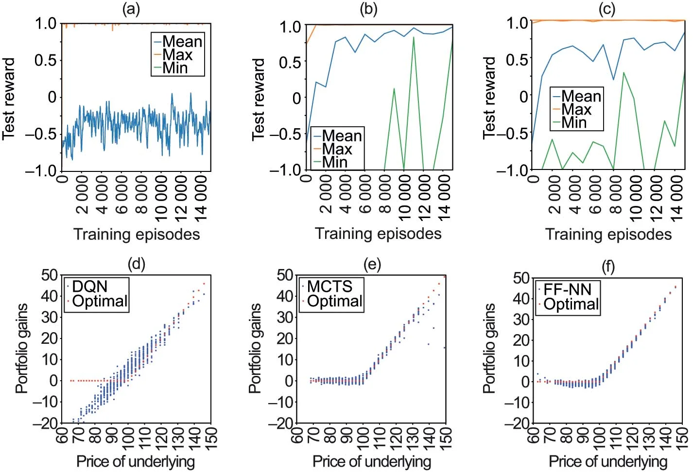
As a first illustration, we compare MCTS with “deep-hedging” (supervised learning) and the DQN for TV hedging without transaction costs (see Example 2.2). We employ the trinomial market model of Table 1. The experiments with the DQN are based on the RLlib open source implementation (Liang et al 2018) of the “Rainbow DQN” of Hessel et al (2018). The hedging environment is available in an open source repository (Szehr 2023b). For supervised learning we train an FF-NN that is optimized simultaneously over the whole sequence of hedging decisions $(n_1,n_2,\mathrm{\dots },n_T)$, which corresponds to a continuous action space. We use a concatenation of 59 shallow NNs (with three layers, each consisting of 32 neurons), where the price and hedge of each training episode become the input for the subsequent episode. The model is described by Buehler et al (2019a), and an implementation is provided in the open source repository (Teichmann 2019). Our comparison is mostly illustrative as model-based RL; model-free RL and supervised learning serve different purposes. Figure 2 compares the training progress over 15 000 samples. The MCTS and FF-NN are retrained every 1000 samples by 10 epochs of batches of size 32. Subsequently, the hedging performance is evaluated on 100 out-of-sample paths. For the DQN we show TensorBoard outputs, where the agent is retrained once samples become available. The graphs in parts (a)–(c) of Figure 2 show the mean, maximum and minimum of the test rewards over a typical training cycle. In these graphs risk-free hedging would correspond to a reward of 1, but in our setting hedging errors occur due to the discretization of time, space and, in the case of DQN and MCTS, actions. The graphs in parts (d)–(f) compare the trained agents by giving the gains of the replicating portfolios on 1000 out-of-sample paths and the value of the option contract at maturity. The underlying takes discrete values because a trinomial market model is employed. The training and runtime performance is poor for the DQN. The reason is that rewards are granted only at option maturity (but see also the work of Cannelli et al (2023), who show that the DQN does not reach the performance of a contextual bandit on P&L hedging). Note that in our implementation DQN receives the same reward signal as MCTS and FF-NN, which differs from previous successful reports on the application of DQN (see, for example, Kolm and Ritter 2019; Cao et al 2021) in that no reward signal is available before maturity.

As a benchmark, Figure 3 shows MCTS’s training progress by providing mean and median rewards computed from 10 independent training cycles.

4.6 Training to perfection

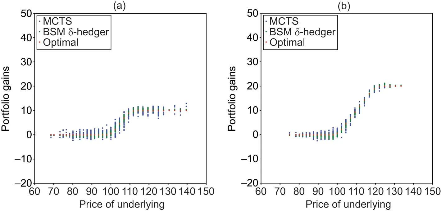
We consider the same MCTS and FF-NN models and the trinomial market model as before. We train until the rewards are maximal and compare the terminal portfolio gains of the respective trading strategies in Figure 4. For illustration, we also show the gains that would have been obtained had the hedger followed the BSM $\delta$-hedging rule instead of MCTS or FF-NN. In the case of FF-NN we grant 100 000 episodes and 50 epochs of training. In the case of MCTS we grant 20 000 samples over 20 training cycles and reinforce the outcome with a further 20 cycles and a sharper reward signal (corresponding to 40 000 samples in total). The graphs in parts (a)–(c) of Figure 4 compare the agents showing the gains of the replicating portfolio on 1000 out-of-sample paths and the value of the option contract at maturity. The graphs in parts (d)–(f) of Figure 4 compare the actions taken by the different agents in the middle of the planning horizon, where the action space is continuous for the $\delta$-hedger and the FF-NN but discrete for MCTS. In the BSM economy risk-free hedging is achieved by the $\delta$-hedge portfolio, but here we are faced with discretization errors. As a consequence, taking action based on the BSM $\delta$-hedging rule is no longer optimal. Figure 4(a) shows that the trading gains from the $\delta$-hedger turn out to be slightly lower than the value of the option. In this experiment the average Euclidean distance between the outcomes of the replicating portfolio and the values of the option contract over 1000 paths turned out to be 0.028 for the $\delta$-hedger, 0.0276 for the FF-NN and 0.0265 for MCTS. The figures for the FF-NN and MCTS are not directly comparable (due to differences in architecture, action spaces, training and test sets, etc), but it is notable that MCTS achieves a comparatively small distance (after a comparatively small number of training samples) despite being restricted to choosing from only 21 possible actions. The distribution of hedges is also most symmetric around the call value for MCTS (see Figure 4(b)). Apparently, MCTS compensates for its restrictions by effectively learning the statistics of the trinomial model. It is also notable that the actions chosen by MCTS (see Figure 4(e)) are very different from BSM and FF-NN hedges.

4.7 Varying reward structures

 

Figure 5: Comparison of the terminal portfolio gains for call spreads. (a) MCTS, K_{\text{1}}=\text{100}, K_{\text{2}}=\text{110}. (b) MCTS, K_{\text{1}}=\text{100}, K_{\text{2}}=\text{120}.

 

 

Figure 6: MCTS training progress for the utility of Examples 2.1 and 2.3. (a) BSM utility. (b) CARA utility, \lambda =\text{1}, \eta =\text{0.01}.

 

 

Figure 7: Comparison of terminal portfolio gains. (a) GBM. (b) Heston model.

 

 

Figure 8: Comparison of FF-NN with MCTS in trinomial model with transaction costs, \lambda =\text{1}. (a) FF-NN accumulated transaction costs. (b) MCTS accumulated transaction costs. (c) FF-NN portfolio gains. (d) MCTS portfolio gains.

 

 

Figure 9: Comparison of FF-NN with MCTS in trinomial model with transaction costs, \lambda =10. (a) FF-NN accumulated transaction costs. (b) MCTS accumulated transaction costs. (c) FF-NN portfolio gains. (d) MCTS portfolio gains.

 

Table 2: Quantitative comparison of FF-NN versus MCTS.

			Average
	Risk	Accumulated	quadratic	Normalized
Agent	average	costs	loss	loss
BSM	$\lambda =\text{1}$	3.30	18.58	0.03397
FF-NN	$\lambda =\text{1}$	0.30	58.32	0.00594
MCTS	$\lambda =\text{1}$	0.22	72.23	0.00583
BSM	$\lambda =\text{10}$	3.18	17.31	0.04048
FF-NN	$\lambda =\text{10}$	0.77	19.96	0.01767
MCTS	$\lambda =\text{10}$	0.61	22.42	0.01730

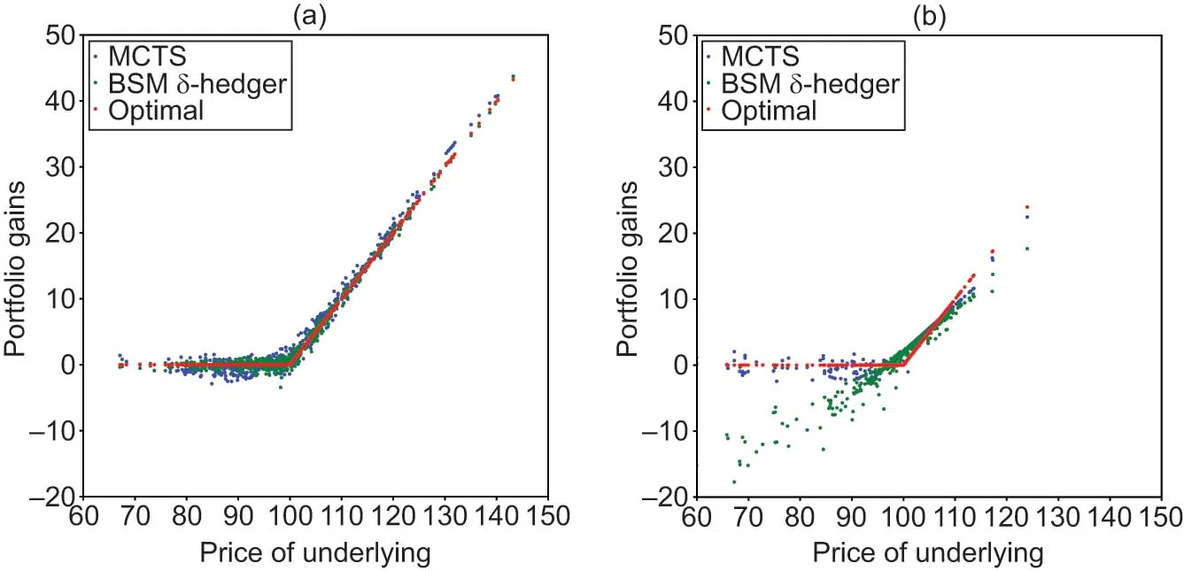
We demonstrate that MCTS remains effective if faced with more general reward signals, including varying contractual payoffs and utility functions. Figure 5 illustrates the application of MCTS for the hedging of call spreads with a payoff of the form $Z_T={(S_T-K_1)}^{+}-{(S_T-K_2)}^{+}$. The portfolio gains of a trained MCTS agent (20 training cycles) are compared with the respective BSM $\delta$-hedge portfolios for two spreads. Figure 6 illustrates the training progress with varying utility functions. The rewards correspond to the utility functions of Examples 2.1 and 2.3 (while the rewards for Example 2.2 are given in Figure 2(b)). For the BSM example, the rewards are accumulated over the training episode, but in each case the whole reward is granted at option maturity. The performance of the CARA investor after training is discussed in Section 4.9.

4.8 Varying underlying models

We demonstrate that MCTS remains effective when applied to hedging on continuous market models. We employ the GBM and Heston models of Table 1. Figure 7 compares the terminal hedging gains of the MCTS agent with the gains of the $\delta$-hedger after 20 training cycles of 1000 episodes.

4.9 Transaction costs

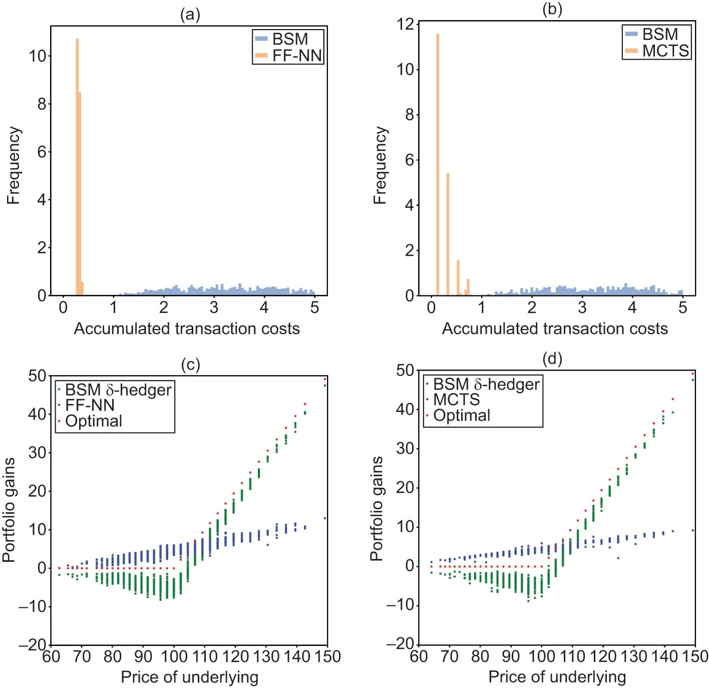
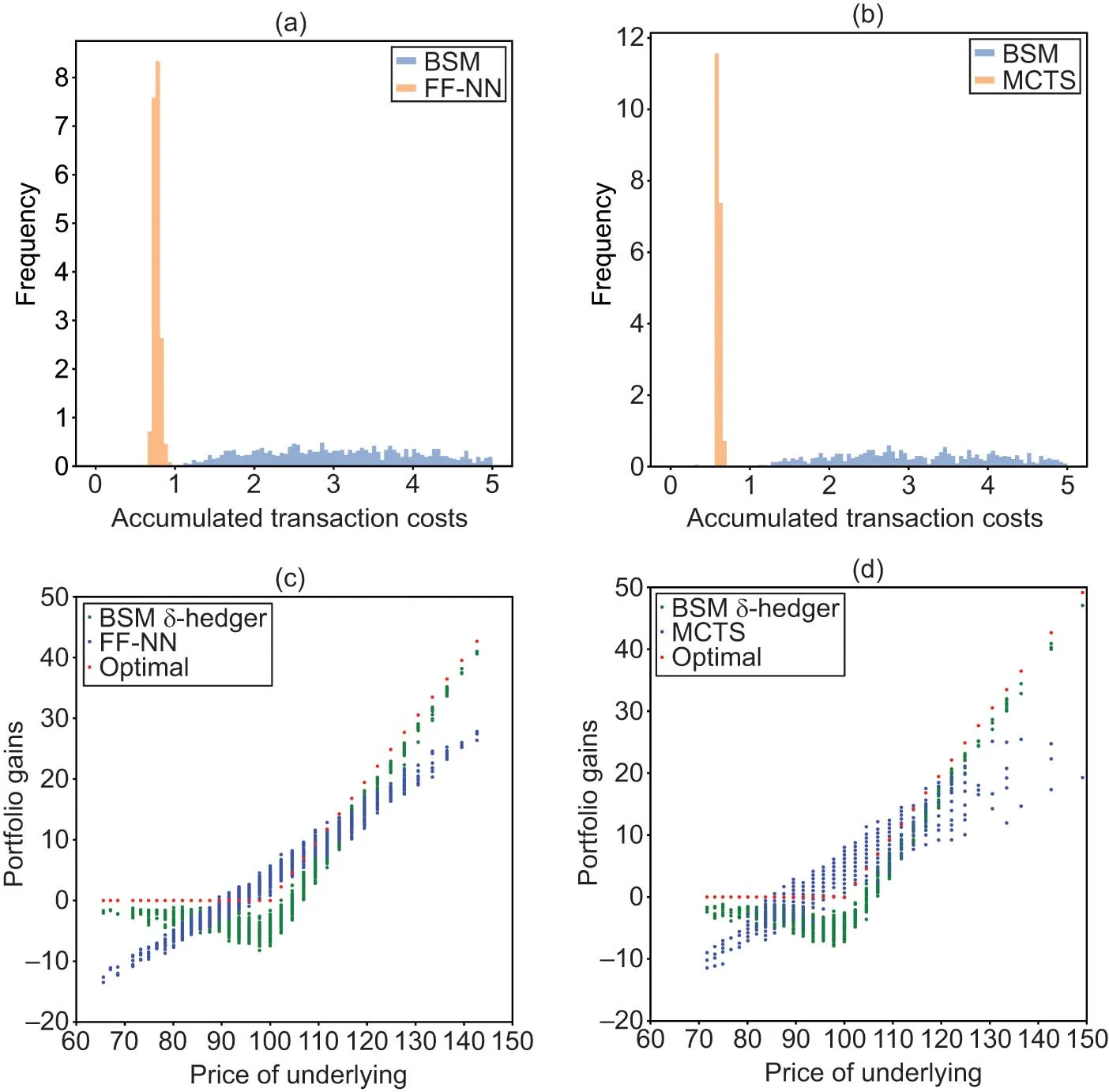
We demonstrate that MCTS remains effective when faced with transaction costs. We compare portfolio gains and accumulated transaction costs from the MCTS and FF-NN models. We consider a CARA investor in a trinomial market with costs of the form $\mathrm{cost}(n_t,n_{t+1},S_t)=-0.01|\mathrm{\Delta }{n}_{t+1}|S_t$ and two levels of risk aversion $\lambda =1,10$. As in Section 4.5, we provide each of the models with 15 training cycles of 1000 episodes and we use 1000 paths for testing. Figure 8 presents the results of our comparison for $\lambda =1$, and Figure 9 for $\lambda =10$. Histograms of transaction costs accumulated over the planning horizon are shown, respectively, in parts (a) and (b). Parts (c) and (d) present the terminal portfolio gains. For comparison, the accumulated costs and portfolio gains of the $\delta$-hedger are also added. Table 2 contains the exact figures obtained from this experiment. The $\delta$-hedger achieves the smallest average Euclidean distance to target option values at the expense of high transaction costs. The smallest normalized loss, and consequently the highest CARA utility, is achieved by MCTS.¹⁵¹⁵ 15 The normalized loss of the CARA investor is $\text{Loss}(X)=1/\lambda (1-{\mathrm{e}}^{-\lambda X/S_0})$. At this stage it should be said that this behavior might be an artifact of the chosen architectures and hyperparameters.¹⁶¹⁶ 16 It is conceivable that the performance of FF-NN could be improved by using a recurrent NN or a long short-term memory network. We leave detailed benchmark comparisons of the overall performance of MCTS versus “deep-hedging” methods for future research.

5 Conclusion

We introduced planning-based reinforcement learning to an important planning problem of financial engineering: the hedging of derivative contracts in incomplete markets. We interpreted this problem as a “game with the world”, where the success of MCTS in a variety of games and general game-play motivated our investigation of this algorithm. We demonstrated the effectiveness of MCTS for hedging with simple contracts, market-models and reward structures. In a setting where rewards are only granted as a consequence of contractual cashflows, we compared the performance of neural MCTS (AlphaZero) with DQN and “deep-hedging” methods. We observed that DQN appears to cope poorly with such reward structures. For MCTS and “deep-hedging” methods we observed an overall comparable performance, but our findings suggest that MCTS has a slightly higher sample efficiency. We leave detailed benchmark comparisons of MCTS versus “deep-hedging” methods for future research. In view of the greater complexity of the MCTS architecture, “deep-hedging” remains the practical choice for simple applications. However, in applications, where gradient-decent optimization converges to a poor local optimum or where limited data is available for training, MCTS’s planning and generalization capability might point to a potential solution.

Declaration of interest

The author reports no conflicts of interest. The author alone is responsible for the content and writing of the paper.

Acknowledgements

Cordial thanks go to Giacomo Del Rio for introducing the author to remote servers, to Matteo Maggiolo for helping the author to run the experiments and to Miroslav Štrupl for reading the manuscript. The author equally wishes to thank the anonymous referees, whose reports led to a significant improvement of the manuscript.

References

• Aase, K. K. (1988). Contingent claims valuation when the security price is a combination of an Ito process and a random point process. Stochastic Processes and Their Applications 28(2), 185–220 (https://doi.org/10.1016/0304-4149(88)90096-8).
• Anthony, T., Tian, Z., and Barber, D. (2017). Thinking fast and slow with deep learning and tree search. In 31st Annual Conference on Neural Information Processing Systems, Guyon, I., Luxburg, U. V., Bengio, S., Wallach, H., Fergus, R., Vishwanathan, S., and Garnett, R. (eds). Advances in Neural Information Processing Systems, Volume 30. Curran Associates, Red Hook, NY.
• Auer, P., Cesa-Bianchi, N., and Fischer, P. (2002). Finite-time analysis of the multiarmed bandit problem. Machine Learning 47, 235–256 (https://doi.org/10.1023/a:1013689704352).
• Barron, E., and Jensen, R. (1990). A stochastic control approach to the pricing of options. Mathematics of Operations Research 15(1), 49–79 (https://doi.org/10.1287/moor.15.1.49).
• Bisi, L., Sabbioni, L., Vittori, E., Papini, M., and Restelli, M. (2020). Risk-averse trust region optimization for reward-volatility reduction. In Proceedings of the Twenty-Ninth International Joint Conference on Artificial Intelligence, pp. 4583–4589. IJCAI (https://doi.org/10.24963/ijcai.2020/632).
• Black, F., and Scholes, M. (1973). The pricing of options and corporate liabilities. Journal of Political Economy 81(3), 637–654 (https://doi.org/10.1086/260062).
• Bouchaud, J.-P., and Sornette, D. (1994). The Black–Scholes option pricing problem in mathematical finance: generalization and extensions for a large class of stochastic processes. Journal de Physique I 4(6), 863–881 (https://doi.org/10.1051/jp1:1994233).
• Boyle, P. (1986). Option valuation using a three-jump process. International Options Journal 3, 7–12.
• Browne, C. B., Powley, E., Whitehouse, D., Lucas, S. M., Cowling, P. I., Rohlfshagen, P., Tavener, S., Perez, D., Samothrakis, S., and Colton, S. (2012). A survey of Monte Carlo tree search methods. IEEE Transactions on Computational Intelligence and AI in Games 4(1), 1–43 (https://doi.org/10.1109/TCIAIG.2012.2186810).
• Buehler, H., Gonon, L., Teichmann, J., and Wood, B. (2019a). Deep hedging. Quantitative Finance 19(8), 1271–1291 (https://doi.org/10.1080/14697688.2019.1571683).
• Buehler, H., Gonon, L., Teichmann, J., Wood, B., Mohan, B., and Kochems, J. (2019b). Deep hedging: hedging derivatives under generic market frictions using reinforcement learning. Research Paper 19-80, Swiss Finance Institute, Zurich (https://doi.org/10.2139/ssrn.3355706).
• Cannelli, L., Nuti, G., Sala, M., and Szehr, O. (2023). Hedging using reinforcement learning: contextual $k$-armed bandit versus $Q$-learning. Journal of Finance and Data Science 9, Paper 100101 (https://doi.org/10.1016/j.jfds.2023.100101).
• Cao, J., Chen, J., Hull, J., and Poulos, Z. (2021). Deep hedging of derivatives using reinforcement learning. Journal of Financial Data Science 3(1), 10–27 (https://doi.org/10.3905/jfds.2020.1.052).
• Chang, H. S., Fu, M. C., Hu, J., and Marcus, S. I. (2005). An adaptive sampling algorithm for solving Markov decision processes. Operations Research 53(1), 126–139 (https://doi.org/10.1287/opre.1040.0145).
• Clewlow, L., and Hodges, S. (1997). Optimal delta-hedging under transactions costs. Journal of Economic Dynamics and Control 21(8–9), 1353–1376 (https://doi.org/10.1016/s0165-1889(97)00030-4).
• Couëtoux, A. (2013). Monte Carlo tree search for continuous and stochastic sequential decision making problems. PhD Thesis, Université Paris Sud–Paris XI. URL: https://theses.hal.science/tel-00927252/.
• Cox, J. C., Ross, S. A., and Rubinstein, M. (1979). Option pricing: a simplified approach. Journal of Financial Economics 7(3), 229–263 (https://doi.org/10.1016/0304-405x(79)90015-1).
• Davis, M. H. A., Panas, V. G., and Zariphopoulou, T. (1993). European option pricing with transaction costs. SIAM Journal on Control and Optimization 31(2), 470–493 (https://doi.org/10.1137/0331022).
• Dean, T., Kaelbling, L. P., Kirman, J., and Nicholson, A. (1995). Planning under time constraints in stochastic domains. Artificial Intelligence 76(1–2), 35–74 (https://doi.org/10.1016/0004-3702(94)00086-G).
• Delbaen, F., and Schachermayer, W. (2006). The Mathematics of Arbitrage. Springer Finance (https://doi.org/10.1007/978-3-540-31299-4).
• Duffie, D. (2001). Dynamic Asset Pricing Theory, 3rd edn. Princeton University Press.
• El Karoui, N., and Quenez, M.-C. (1995). Dynamic programming and pricing of contingent claims in an incomplete market. SIAM Journal on Control and Optimization 33(1), 29–66 (https://doi.org/10.1137/s0363012992232579).
• Finnsson, H., and Björnsson, Y. (2008). Simulation-based approach to general game playing. In Proceedings of the 23rd National Conference on Artificial Intelligence, pp. 259–264. ACM Press, New York. URL: https://cdn.aaai.org/AAAI/2008/AAAI08-041.pdf.
• Föllmer, H., and Sondermann, D. (1986). Hedging of non-redundant contingent claims. In Contributions to Mathematical Economics – In Honour of Gérard Debrev, Hildenbrand, W., and Mas-Colell, A. (eds), pp. 205–223. North Holland, Amsterdam.
• Genesereth, M., and Björnsson, Y. (2013). The international general game playing competition. AI Magazine 34(2), 107–111 (https://doi.org/10.1609/aimag.v34i2.2475).
• Guo, X., Singh, S., Lee, H., Lewis, R. L., and Wang, X. (2014). Deep learning for real-time Atari game play using offline Monte-Carlo tree search planning. In Proceedings of the 27th International Conference on Neural Information Processing Systems, Volume 2, Ghahramani, Z., Welling, M., Cortes, C., Lawrence, N., and Weinberger, K. (eds). Advances in Neural Information Processing Systems, Volume 27. MIT Press, Cambridge, MA. URL: https://proceedings.neurips.cc/paper_files/paper/2014/file/8bb88f80d334b1869781beb89f7b73be-Paper.pdf.
• Halperin, I. (2017). QLBS: Q-learner in the Black–Scholes(–Merton) worlds. Preprint (arXiv:1712.04609) (https://doi.org/10.48550/arXiv.1712.04609).
• Hansen, E. A., and Zilberstein, S. (2001). LAO${ }^{*}$: a heuristic search algorithm that finds solutions with loops. Artificial Intelligence 129(1–2), 35–62 (https://doi.org/10.1016/S0004-3702(01)00106-0).
• Hessel, M., Modayil, J., van Hasselt, H., Schaul, T., Ostrovski, G., Dabney, W., Horgan, D., Piot, B., Azar, M., and Silver, D. (2018). Rainbow: combining improvements in deep reinforcement learning. Proceedings of the AAAI Conference on Artificial Intelligence 32(1), 3215–3222 (https://doi.org/10.1609/aaai.v32i1.11796).
• Hodges, S., and Neuberger, A. (1989). Option replication of contingent claims under transactions costs. Review of Futures Markets 2(8), 222–239.
• Hull, J., and White, A. (1987). The pricing of options on assets with stochastic volatilities. Journal of Finance 42(2), 281–300 (https://doi.org/10.1111/j.1540-6261.1987.tb02568.x).
• Kearns, M., Mansour, Y., and Ng, A. Y. (2002). A sparse sampling algorithm for near-optimal planning in large Markov decision processes. Machine Learning 49(2/3), 193–208 (https://doi.org/10.1023/A:1017932429737).
• Kim, B., Lee, K., Lim, S., Kaelbling, L., and Lozano-Perez, T. (2020). Monte Carlo tree search in continuous spaces using Voronoi optimistic optimization with regret bounds. Proceedings of the AAAI Conference on Artificial Intelligence 34(6), 9916–9924 (https://doi.org/10.1609/aaai.v34i06.6546).
• Kocsis, L., and Szepesvári, C. (2006). Bandit based Monte-Carlo planning. In Machine Learning: ECML 2006, Fürnkranz, J., Scheffer, T., and Spiliopoulou, M. (eds), pp. 282–293. Lecture Notes in Computer Science, Volume 4212. Springer (https://doi.org/10.1007/11871842_29).
• Kocsis, L., Szepesvári, C., and Willemson, J. (2006). Improved Monte-Carlo search. Working Paper, MTA SZTAKI, Budapest. URL: http://old.sztaki.hu/{~}szcsaba/papers/cg06-ext.pdf.
• Kolm, P. N., and Ritter, G. (2019). Dynamic replication and hedging: a reinforcement learning approach. Journal of Financial Data Science 1(1), 159–171 (https://doi.org/10.2139/ssrn.3281235).
• Lee, J., Jeon, W., Kim, G.-H., and Kim, K.-E. (2020). Monte-Carlo tree search in continuous action spaces with value gradients. Proceedings of the AAAI Conference on Artificial Intelligence 34(4), 4561–4568 (https://doi.org/10.1609/aaai.v34i04.5885).
• Liang, E., Liaw, R., Nishihara, R., Moritz, P., Fox, R., Goldberg, K., Gonzalez, J., Jordan, M., and Stoica, I. (2018). RLlib: abstractions for distributed reinforcement learning. Proceedings of Machine Learning Research 80, 324–333. URL: https://proceedings.mlr.press/v80/liang18b.pdf.
• Merton, R. C. (1973). Theory of rational option pricing. Bell Journal of Economics and Management Science 4(1), 141–183 (https://doi.org/10.2307/3003143).
• Merton, R. C. (1990). Continuous-Time Finance. Blackwell, Cambridge, MA.
• Mnih, V., Kavukcuoglu, K., Silver, D., Graves, A., Antonoglou, I., Wierstra, D., and Riedmiller, M. (2013). Playing Atari with deep reinforcement learning. Preprint (arXiv:1312.5602) (https://doi.org/10.48550/arXiv.1312.5602).
• Péret, L., and Garçia, F. (2004). On-line search for solving Markov decision processes via heuristic sampling. In Proceedings of the 16th Eureopean Conference on Artificial Intelligence, ECAI’2004, Including Prestigious Applicants of Intelligent Systems, PAIS 2004, pp. 530–534. URL: https://frontiersinai.com/ecai/ecai2004/ecai04/pdf/p0530.pdf.
• Pérez-Liébana, D., Lucas, S. M., Gaina, R. D., Togelius, J., Khalifa, A., and Liu, J. (2019). General Video Game Artificial Intelligence. Synthesis Lectures on Games and Computational Intelligence, Volume 3. Morgan & Claypool Publishers (https://doi.org/10.1007/978-3-031-02122-0).
• Ramanujan, R., Sabharwal, A., and Selman, B. (2011). On the behavior of UCT in synthetic search spaces. In Proceedings of the ICAPS Conference on Artificial Intelligence. URL: https://icaps11.icaps-conference.org/proceedings/mcts/ramanujan-et-al.pdf.
• Schäl, M. (1994). On quadratic cost criteria for option hedging. Mathematics of Operations Research 19(1), 121–131 (https://doi.org/10.1287/moor.19.1.121).
• Schweizer, M. (1995). Variance-optimal hedging in discrete time. Mathematics of Operations Research 20(1), 1–32 (https://doi.org/10.1287/moor.20.1.1).
• Shafer, G., and Vovk, V. (2001). Probability and Finance: It’s Only a Game! Wiley (https://doi.org/10.1002/0471249696).
• Silver, D., Schrittwieser, J., Simonyan, K., Antonoglou, I., Huang, A., Guez, A., Hubert, T., Baker, L., Lai, M., Bolton, A., Chen, Y., Lillicrap, T., Hui, F., Sifre, L., van den Driessche, G., Graepel, T., and Hassabis, D. (2017). Mastering the game of Go without human knowledge. Nature 550, 354–359 (https://doi.org/10.1038/nature24270).
• Silver, D., Hubert, T., Schrittwieser, J., Antonoglou, I., Lai, M., Guez, A., Lanctot, M., Sifre, L., Kumaran, D., Graepel, T., Lillicrap, T., Simonyan, K., and Hassabis, D. (2018). A general reinforcement learning algorithm that masters chess, shogi and Go through self-play. Science 362(6419), 1140–1144 (https://doi.org/10.1126/science.aar6404).
• Sutton, R. S., and Barto, A. G. (2018). Reinforcement Learning: An Introduction. MIT Press, Cambridge, MA.
• Świechowski, M., Godlewski, K., Sawicki, B., and Mańdziuk, J. (2022). Monte Carlo tree search: a review of recent modifications and applications. Artificial Intelligence Review 56, 2497–2562 (https://doi.org/10.1007/s10462-022-10228-y).
• Szehr, O. (2023a). Minimal AlphaZero hedger. URL: https://github.com/plan64/minimalHedger_AlphaZero.
• Szehr, O. (2023b). MinimalHedger_DQN_RLlib. GitHub Repository. URL: https://github.com/plan64/minimalHedger_DQN_RLlib.
• Teichmann, J. (2020). Deep hedging. URL: https://gist.github.com/jteichma.
• Torrado, R., Bontrager, P., Togelius, J., Liu, J., and Perez-Liebana, D. (2018). Deep reinforcement learning for general video game AI. Preprint (arXiv:1806.02448) (https://doi.org/10.48550/arXiv.1806.02448).
• Vanderbei, R. (1996). Optimal sailing strategies. Unpublished Lecture Notes, Statistics and Operations Research Program. University of Princeton, Princeton, NJ.
• Vittori, E., Trapletti, E., and Restelli, M. (2020). Option hedging with risk averse reinforcement learning. In Proceedings of the First ACM International Conference on AI in Finance, pp. 1–8. ACM Press, New York (https://doi.org/10.1145/3383455.3422532).
• Watkins, C. J. C. H., and Dayan, P. (1992). $Q$-learning. Machine Learning 8, 279–292 (https://doi.org/10.1007/BF00992698).
• Xiao, C., Huang, R., Mei, J., Schuurmans, D., and Müller, M. (2019). Maximum entropy Monte-Carlo planning. In Proceedings of the 33rd International Conference on Neural Information Processing Systems, Wallach, H., Larochelle, H., Beygelzimer, A., d’Alché-Buc, F., Fox, E., and Garnett, R. (eds). Advances in Neural Information Processing Systems, Volume 32. Curran Associates, Red Hook, NY.
• Zakamouline, V. I. (2006). European option pricing and hedging with both fixed and proportional transaction costs. Journal of Economic Dynamics and Control 30(1), 1–25 (https://doi.org/10.1016/j.jedc.2004.11.002). 

Download PDF

• Keywords
• Derivatives
• Hedging
• Monte Carlo simulation
• Pricing
• Original research