Risk management for private equity funds

Axel Buchner

Abstract

Although risk management has been explored thoroughly in financial modeling for over three decades, there is still a limited understanding of how to correctly quantify and manage the risks of investing in private equity, which continues to hinder our understanding of the risks associated with other traditional asset classes. This paper develops a comprehensive risk management framework for private equity fund investments, which captures the three main sources of risks that private equity investors face when investing in the asset class: market risk, liquidity risk and cashflow risk. Underlying the framework is a stochastic model for the value and cashflow dynamics of private equity funds, which allows us to derive three dynamic risk measures for private equity fund investments: value-at-risk, liquidity-adjusted value-at-risk and cashflow-at-risk. The model is calibrated with historical data of buyout funds, and the dynamics of the developed risk measures are illustrated for a single fund investment using Monte Carlo simulations. A model extension also studies the dynamics of the risk measures for portfolios of funds and develops a novel dynamic commitment strategy. Finally, sensitivity analyses show the impact of changes in the main model parameters on risk measures.

Download PDF Appendix 1

Introduction

1 Introduction

Private equity continues to grow in importance as an asset class, as investors seek diversification benefits relative to traditional stock and bond holdings. In particular, large institutional investors, such as insurance companies, endowment and pension funds, are allocating increasing portions of their overall investment portfolios to private equity. Most of these investments are intermediated through funds, because entering, managing and exiting direct private equity investments requires high levels of expertise and experience. Despite the increasing importance of private equity as an asset class, our understanding of how investors can adequately measure and manage the risks of these investments remains limited and continues to lag considerably behind that of other traditional asset classes. The aim of this paper is to develop what is, to the best of our knowledge, the first comprehensive risk management framework for private equity fund investments.

Private equity funds have at least two key institutional features that differentiate them from traditional investments in traded stocks or bonds and make risk management a challenging task. First, private equity fund investments are illiquid and long term. Private equity funds typically have maturities of ten to fourteen years, and secondary markets for private equity fund positions are still highly inefficient, making it costly for investors to sell their positions. Second, private equity fund investments involve specific dynamics of capital drawdowns and distributions. The private equity fund investor first makes an initial capital commitment and later transmits specific amounts of capital to the general partner in response to capital calls (or capital drawdowns). The timing and size of the capital calls are not known until they are announced, and usually there is a substantial lag between the time at which capital is committed to a fund and the time at which that capital is actually drawn for investment. In addition, cash payouts by private equity funds are also uncertain, although they are significant, because of the bounded life cycle of the funds. Thus, the invested capital changes dynamically over the lifetime of a fund, and private equity fund investments require active cashflow management of capital calls and distributions.

Taking into account these special features, a risk management framework for private equity fund investments has to capture three main sources of risk.

1. (i)

   Market risk: the risk of losses in the market prices of the portfolio companies held by a fund exposes investors to market risk.

2. (ii)

   Liquidity risk: the illiquidity of private equity partnership interests exposes investors to asset liquidity risk associated with selling positions in the secondary markets at potentially large and ex ante uncertain discounts on a fund’s net asset value.

3. (iii)

   Funding (or cashflow) risk: the unpredictable timing and magnitude of fund cashflows pose funding and cashflow risks to investors. In particular, capital commitments are contractually binding, and defaulting on these payments can result in the loss of the entire private equity partnership interest.

The framework developed in this paper allows these three main sources of risk to be addressed using distinct risk measures. Underlying the risk management framework is a model of the dynamics of private equity funds with three main components corresponding to the essential phases of the private equity fund life cycle: the drawdowns from the committed capital paid into the fund; the performance of the investments effected by the fund; and the distributions of dividends and proceeds taken out of the fund. Effectively, a standard lognormal process that is correlated with aggregate stock market returns is used for the dynamics of the investment value. Capital drawdowns and distributions are modeled by two stochastic processes for the dynamics of the rates of drawdowns and repayments. Taking into account that the speed of capital drawdowns and distributions may be affected by the overall state of the economy, the model also incorporates the possibility that the drawdown and repayment rates are correlated with aggregate stock market returns. Given this stochastic model, in this paper we propose three risk measures for private equity fund investments.

Market risk is captured by using a value-at-risk (VaR) approach, which has become the standard measure used by financial analysts to quantify this risk (see Jorion 2001).¹¹In addition to their risk management applications, VaR measures are also important for regulatory capital requirements. In particular, the Basel Committee on Banking Supervision at the Bank for International Settlements requires financial institutions such as banks and investment firms to meet capital requirements based on VaR estimates. Generally, VaR is defined as the maximum potential loss in value of a portfolio of financial instruments with a given probability over a certain horizon. In other words, it is a number indicating how much a financial institution can lose with a given probability over a given time horizon. Standard VaR implementations assume a static setting in which the mix of a position is unchanged over time, ie, no cash inflows or outflows occur over the VaR horizon. In contrast, the VaR approach presented here is dynamic in the sense that it also takes into account that the investor’s risk exposure varies over the life cycle of the fund with stepwise capital drawdowns and distributions.

The VaR measure developed is based on the implicit assumption that an investor can at any time sell their position in the fund at the fund’s current net asset value. In reality, stakes in private equity funds are highly illiquid and can typically only be sold at some discount on the secondary private equity markets. In order to account for this form of liquidity risk, the VaR calculation is extended to a liquidity-adjusted VaR (LVaR). The main idea of this is to include secondary markets discounts as an exogenous liquidity cost in the VaR calculation. By capturing the unpredictable nature of secondary market discount dynamics, discounts are thereby modeled using a mean-reverting Ornstein–Uhlenbeck process, which is also assumed to be correlated with aggregate stock market returns.

Finally, to capture funding (or cashflow) risk, the paper introduces a cashflow-at-risk (CFaR) measure. This measure is defined as the change (loss) in the investor’s cash position, which is only exceeded with some given probability, over a given time horizon. This measure is also dynamic and its interpretation changes with the stages in the fund’s life cycle.

After calibrating the model such that parameters correspond to an investment in a typical buyout fund, the risk measures developed are illustrated using Monte Carlo simulations. The results underline that there are specific patterns of private equity in VaR dynamics that a sensible risk management framework for fund investors must take into account. In particular, the VaR initially rises sharply up to some fixed time horizon, but then peaks and decreases to zero over the fund’s lifetime. This behavior is consistent with the typical life cycle of private equity funds. As the fund gradually draws down capital and builds up the investment portfolio, the investor’s risk exposure increases markedly. After the maximum level has been reached, the fixed-horizon VaR decays rapidly toward zero as capital distributions of the fund decrease the investor’s risk exposure stepwise.

A comparison between the simulated VaR and LVaR measures highlights that the effects of illiquidity on the investor’s risk exposure over the life of a fund can be substantial. However, the numerical results also show that illiquidity only increases the investor’s risk exposure if the time horizon under consideration is shorter than the fund’s total remaining lifetime, as liquidity risk is fully resolved with the final liquidation of a fund. The effects of liquidity risk are thus investor specific. For investors facing the risk of being forced to sell their private equity positions on the secondary markets due to a surprise liquidity shock during the fund lifetime, ignoring liquidity risk can lead to substantially underestimated risk figures. In contrast, for investors with sufficient cash reserves and a low probability of facing surprise liquidity shocks, liquidity risk is only of minor importance.

The dynamics of the simulated CFaR measure further illustrate how cashflow risk changes with the development stage of the fund. In the early stages of a fund’s life, when the fund starts to call capital from the investors, CFaR is large and gives a measure of funding risk, ie, the maximum amount of cash that an investor must hold in reserve in order to be able to meet capital calls with a given probability. Later in the fund’s life, when it starts to gradually exit its portfolio companies and returns the proceeds to the investors, CFaR decreases and gives a measure of distribution risk, ie, the negative value of CFaR gives an indication of the minimum amount of cash distributed by the private equity fund over some given time horizon with some given probability.

Finally, our model and numerical analysis are extended to a portfolio context. We consider both a static portfolio and a dynamic portfolio of private equity funds. In the static portfolio case, we assume that the capital commitment to each fund is set at the constitution of the portfolio and remains unchanged thereafter. The numerical results highlight how portfolio diversification can help to reduce the VaR and CFaR measures. As expected, the reduction in risk increases with the number of portfolio funds. In the dynamic portfolio case, we develop a novel dynamic commitment strategy for private equity fund investors who aim to attain a constant amount of capital invested in private equity funds over time. The numerical results show that this dynamic strategy leads to a fixed-horizon VaR that converges to a constant level over time. The results additionally illustrate that building up a private equity portfolio from scratch can require significant amounts of time, and usually involves some degree of initial overcommitment.

This paper is related to studies that evaluate the risk and return characteristics or cashflow dynamics of private equity investments. Important research in this area includes that by Cochrane (2005), Kaplan and Schoar (2005), Ljungqvist et al (2008), Phalippou and Gottschalg (2009), Korteweg and Sorensen (2010), Robinson and Sensoy (2011), Driessen et al (2012), Ang et al (2013), Ewens et al (2013), Harris et al (2014) and Hochberg et al (2014). None of these studies, however, develops an integrated risk model for private equity investments. The only scientific paper in the area of risk management is a study by Bongaerts and Charlier (2009), who apply existing credit risk models to individual private equity investments.²²There are several papers by industry analysts on the issue of risk management (see, for example, Diller and Herger 2008). Most of these simply perform ad hoc bootstrap simulations of fund internal rates of return (IRRs) or multiples using historical cashflow data. However, their model is difficult to calibrate and fails to address liquidity and cashflow risks of private equity fund investments. We are unaware of any other study that develops a risk model for private equity investments that captures market, liquidity and cashflow risk using standard VaR measures. Developing a model that is sufficiently tractable to accurately quantify these risks is the main contribution of this paper.

The remainder of this paper is organized as follows. Section 2 presents the model of the dynamics of private equity funds. Section 3 develops the three risk measures. Section 4 shows how these risk measures can be estimated using Monte Carlo simulations. Section 5 presents the results of the model calibration and of the numerical model analysis. Section 6 extends the model and numerical analysis to a portfolio context. Section 7 concludes. Details of the model calibration are outlined in Appendixes A and B online.

2 The model

This section develops the model used to derive the risk measures of private equity funds. The model is formulated in a continuous-time framework. It is assumed that all random variables introduced in the following are defined on a probability space $(\mathrm{\Omega },ℱ,\mathbb{P})$, and that all random variables indexed by $t$ are measurable with respect to the filtration $\{{ℱ}_t\}$, representing the information commonly available to all investors.

2.1 Private equity fund dynamics

Following the typical construction of private equity funds, modeling the dynamics of private equity funds requires modeling of the three main components: investment value, capital drawdowns and return repayments.

2.1.1 Investment value

The first step in modeling private equity funds is characterizing value dynamics. Consider a fund with a total legal lifetime given by $T_{\mathrm{l}}$. Let $V_t$ denote the value of the fund’s investment portfolio at time $t$; cumulated capital drawdowns from the limited partners (LPs) up to time $t$ are represented by $D_t$, and cumulated capital distributions to the LPs up to time $t$ are represented by $R_t$. To keep things simple, it is assumed that the return on any cashflow invested in the fund can be described by a normal distribution with constant mean, constant volatility and a constant correlation with aggregate stock market returns.

Assumption 2.1.

The dynamics of the fund value, $V_t$, under the objective probability measure $\mathbb{P}$ can be described by the stochastic process $\mathrm{\{}{V}_t\mathrm{,}\mathrm{0}\mathrm{\le }t\mathrm{\le }{T}_{\mathrm{l}}\mathrm{\}}$:

$$\mathrm{d}{V}_t=V_t({\mu }_V\mathrm{d}t+{\beta }_V{\sigma }_M\mathrm{d}{B}_{M,t}+{\sigma }_{\epsilon }\mathrm{d}{B}_{\epsilon ,t})+\mathrm{d}{D}_t-\mathrm{d}{R}_t,$$

(2.1)

where ${\mu }_V\mathrm{>}\mathrm{0}$ is the mean rate of return, ${\sigma }_M\mathrm{>}\mathrm{0}$ is the return volatility of the aggregate stock market, ${\beta }_V$ is the market beta of the fund and ${\sigma }_{\epsilon }\mathrm{>}\mathrm{0}$ is idiosyncratic volatility; $B_{M\mathrm{,}t}$ is a standard Brownian motion driving aggregate stock market returns³³It is implicitly assumed here that aggregate stock market dynamics, $M_t$, can be described by a standard geometric Brownian motion given by $\mathrm{d}\mathit{}{M}_t\mathrm{=}{\mu }_M\mathit{}{M}_t\mathit{}\mathrm{d}\mathit{}t\mathrm{+}{\sigma }_M\mathit{}{M}_t\mathit{}\mathrm{d}\mathit{}{B}_{M\mathrm{,}t}$, with ${\mu }_M\mathrm{>}\mathrm{0}$ being the mean rate of return, and ${\sigma }_M\mathrm{>}\mathrm{0}$ being the return volatility. and $B_{\epsilon \mathrm{,}t}$ is a second Brownian motion, representing idiosyncratic shocks, ie, $\mathrm{d}\mathit{}{B}_{M\mathrm{,}t}\mathit{}\mathrm{d}\mathit{}{B}_{\epsilon \mathrm{,}t}\mathrm{=}\mathrm{0}$.

This specification of the value dynamics is straightforward. The first term on the right-hand side of the equation, $V_t({\mu }_V\mathrm{d}t+{\beta }_V{\sigma }_M\mathrm{d}{B}_{M,t}+{\sigma }_{\epsilon }\mathrm{d}{B}_{\epsilon ,t})$, states that the instantaneous change in value of a private equity fund is due to the performance of the investment already in place at time $t$. Investments in place are assumed to have normally distributed returns with constant mean given by ${\mu }_V$ and a total variance given by ${\sigma }_V^2={\beta }_V^2{\sigma }_M^2+{\sigma }_{\epsilon }^2$, where ${\beta }_V^2{\sigma }_M^2$ represents systematic variance and ${\sigma }_{\epsilon }^2$ is idiosyncratic variance. This specification takes into consideration the important possibility that private equity fund investment returns and aggregate stock market returns are (potentially highly) correlated with a coefficient of correlation given by ${\rho }_V={\beta }_V{\sigma }_M/{\sigma }_V$. Private equity fund managers receive both a fixed annual management fee, typically 1.5–2.5% of the committed capital, and a performance-based incentive fee (carried interest), typically 20% of capital gains. These fees are incorporated implicitly in (2.1) by defining ${\mu }_V$ to be the expected fund return after all fee components. Hence, it is assumed in the model that fees simply decrease expected fund returns.

The second and third terms on the right-hand side of (2.1) show that fund values are augmented by instantaneous capital drawdowns, $\mathrm{d}{D}_t$, and decreased by instantaneous capital distributions, $\mathrm{d}{R}_t$. By including $\mathrm{d}{D}_t$ and $\mathrm{d}{R}_t$ in (2.1) we take into account the fact that private equity fund investments typically involve stepwise capital drawdowns and generate substantial intermediate capital distributions during the bounded fund’s life cycle. Note that capital distribution (whether in the form of cash or of marketable securities) is directly distributed to the investors as a fund gradually exits its investments. Therefore, capital distributions simply decrease the fund value $V_t$, and there is no need to impose any assumption on the reinvestment of intermediate cashflows.

An important additional feature of the model is that it allows a fund to earn a risk-adjusted excess return, called alpha. Formally, this excess return after fees is defined as

$${\alpha }_V={\mu }_V-r_{\mathrm{f}}-{\beta }_V({\mu }_M-r_{\mathrm{f}}),$$

(2.2)

where ${\mu }_M>0$ is the mean rate of return of the aggregate stock market and $r_{\mathrm{f}}$ is the constant risk-free rate. Intuitively, this alpha is the risk-adjusted (after fee) excess return of the portfolio companies owned and managed by the private equity fund. This excess return may arise from improved governance or from the general partner (GP) being a skillful manager (see, for example, Sorensen et al 2014).

2.1.2 Capital drawdowns

To model capital drawdowns, it is assumed that the fund has an initial committed capital given by $C_0$ and a total commitment period (ie, the period over which capital drawdowns can occur) given by $T_{\mathrm{c}}$ (with $T_{\mathrm{c}}\le T_{\mathrm{l}}$). We assume that at time $t$ capital is drawn from the remaining undrawn committed capital, ie, $C_0-D_t$, at some stochastic rate ${\delta }_t$.

Assumption 2.2.

The dynamics of the cumulated capital drawdowns, $D_t$, can be described by the ordinary differential equation

$$\mathrm{d}{D}_t={\delta }_t(C_0-D_t)1_{\{0\le t\le T_{\mathrm{c}}\}}\mathrm{d}t,$$

(2.3)

where ${\mathrm{1}}_{\mathrm{\{}\mathrm{\cdot }\mathrm{\}}}$ is an indicator function. The fund’s drawdown rate ${\delta }_t$ is assumed to follow a stochastic process $\mathrm{\{}{\delta }_t\mathrm{,}\mathrm{0}\mathrm{\le }t\mathrm{\le }{T}_{\mathrm{c}}\mathrm{\}}$ defined by

$${\delta }_t=\delta +{\sigma }_{\delta }{B}_{\delta ,t},$$

(2.4)

where $\delta \mathrm{>}\mathrm{0}$ is the mean of the drawdown rate and ${\sigma }_{\delta }\mathrm{>}\mathrm{0}$ reflects the volatility of the drawdown rate; $B_{\delta \mathrm{,}t}$ is a third standard Brownian motion, for which it is assumed that $\mathrm{d}\mathit{}{B}_{\delta \mathrm{,}t}\mathit{}\mathrm{d}\mathit{}{B}_{M\mathrm{,}t}\mathrm{=}{\rho }_{\delta }\mathit{}\mathrm{d}\mathit{}t$ and $\mathrm{d}\mathit{}{B}_{\delta \mathrm{,}t}\mathit{}\mathrm{d}\mathit{}{B}_{\epsilon \mathrm{,}t}\mathrm{=}\mathrm{0}$. In order to avoid negative drawdown rates, ${\delta }_t^{\mathrm{+}}\mathrm{=}\max \mathit{}\mathrm{(}{\delta }_t\mathrm{,}\mathrm{0}\mathrm{)}$ is used in the model implementation.

In most cases, capital drawdowns of private equity funds are concentrated in the first few years (or even quarters) of a fund’s life. After high initial investment activity, drawdowns of private equity funds are carried out at a declining rate, as fewer new investments are made, and follow-on investments are spread out over a number of years. This typical time-pattern is well reflected in the structure of (2.3), which implies that initially high capital drawdowns at the start of a fund decrease exponentially over the commitment period, $T_{\mathrm{c}}$. Under this modeling framework, cumulated drawdowns, $D_t$, can also never exceed the total committed capital, $C$. At the same time the model allows for a certain fraction of $C$ not to be drawn, as the commitment period $T_{\mathrm{c}}$ acts as a cut-off point for capital drawdowns. Finally, the model also incorporates the important possibility that the drawdown speed has a nonzero correlation ${\rho }_{\delta }$ with aggregate stock market returns.

2.1.3 Capital distributions

The final step in modeling private equity funds is characterizing the dynamics of the capital distributions. Recognizing that the size and timing of repayments depend on the performance of the fund’s investment portfolio, it is assumed that capital distributions at time $t$ occur at a stochastic rate ${\nu }_t$ from the total investment portfolio value $V_t$ of the fund.

Assumption 2.3.

The dynamics of the cumulated capital distributions, $R_t$, can be described by

(2.5)

The fund’s distribution rate ${\nu }_t$ is assumed to follow a stochastic process $\mathrm{\{}{\nu }_t\mathrm{,}\mathrm{0}\mathrm{\le }t\mathrm{\le }{T}_{\mathrm{l}}\mathrm{\}}$ with specification

$${\nu }_t=\nu t+{\sigma }_{\nu }{B}_{\nu ,t},$$

(2.6)

with constants $\nu \mathrm{,}{\sigma }_{\nu }\mathrm{>}\mathrm{0}$; $B_{\nu \mathrm{,}t}$ is a fourth standard Brownian motion for which it is assumed that $\mathrm{d}\mathit{}{B}_{\nu \mathrm{,}t}\mathit{}\mathrm{d}\mathit{}{B}_{M\mathrm{,}t}\mathrm{=}{\rho }_{\nu }\mathit{}\mathrm{d}\mathit{}t$ and $\mathrm{d}\mathit{}{B}_{\nu \mathrm{,}t}\mathit{}\mathrm{d}\mathit{}{B}_{\epsilon \mathrm{,}t}\mathrm{=}\mathrm{0}$. In order to avoid negative distributions rates, ${\nu }_t^{\mathrm{+}}\mathrm{=}\max \mathit{}\mathrm{(}{\nu }_t\mathrm{,}\mathrm{0}\mathrm{)}$ is used in the model implementation.

The ordinary differential equation for in (2.5) illustrates that capital repayments occur at some rate ${\nu }_t$ from the investment value. This essentially means assuming a dividend process for private equity funds during their lifetimes, similar to the specification used by Takahashi and Alexander (2002) and Malherbe (2004). Moreover, the assumption that the distribution rate dynamics can be described by the Lévy process given in (2.6) is plausible because this specification reflects well the typical life cycle of private equity fund investments, where (average) capital distributions are low at the beginning and increase over the bounded life of the fund as more and more investments are gradually exited. This behavior can easily be inferred from the unconditional expectation of (2.6), $E[{\nu }_t]=\nu t$, which increases linearly over time. In addition, by allowing for a nonzero correlation, $|{\rho }_{\nu }|\le 1$, between changes in the distribution rate and aggregate stock market returns, we incorporate the important possibility that the overall state of the economy (or stock market) affects the speed of capital distributions. For instance, if $1\ge {\rho }_{\nu }>0$, then fast capital distributions will become more likely during stock market booms. Finally, the integral specification for $R_t$ in (2.5) takes into account that a private equity fund is fully liquidated at $T_{\mathrm{l}}$, the end of its legal lifetime. Therefore, cumulated capital distributions over the entire life of a fund must also include the final liquidation proceeds of the fund’s assets at maturity, $T_{\mathrm{l}}$.

2.2 Investor’s position

To define the dynamics of an investor’s position when investing in a private equity fund, assume that undrawn capital commitments, $C_0-D_t$, remain invested at some constant (risk-free) rate $r_{\mathrm{c}}$ until they are actually drawn by the fund management, and that intermediate capital distributions are reinvested at the rate $r_{\mathrm{c}}$ for the remaining lifetime of the fund. As above, let $V_t$ be the net asset value of a private equity fund investment at time $t$ for a given initial commitment $C_0$. In addition, denote by $C_t$ the investor’s cash position at time $t$. Then, the value of the investor’s position at time $t$ is given by $P_t\equiv V_t+C_t$, which reflects that the investor’s position is formed of the net asset value of the private equity fund investment and of their cash holdings. The dynamics of $V_t$ and $C_t$ are given by

	$\mathrm{d}{V}_t$	$=V_t({\mu }_V\mathrm{d}t+{\beta }_V{\sigma }_M\mathrm{d}{B}_{M,t}+{\sigma }_{\epsilon }\mathrm{d}{B}_{\epsilon ,t})+\mathrm{d}{D}_t-\mathrm{d}{R}_t,$		(2.7)
	$\mathrm{d}{C}_t$	$=C_t{r}_{\mathrm{c}}\mathrm{d}t-\mathrm{d}{D}_t+\mathrm{d}{R}_t,$		(2.8)

with $V_0=0$ and $C_0>0$. Equations (2.7) and (2.8) show that capital drawdowns ($\mathrm{d}{D}_t$) decrease the value $C_t$, as the investor has to reduce their cash holdings to meet capital calls, whereas those increase the net asset value $V_t$ of the fund. In contrast, capital distributions ($\mathrm{d}{R}_t$) of a private equity fund decrease the net asset value $V_t$ and increase the value of $C_t$, as they are assumed to be recommitted to private equity funds.

From (2.7) and (2.8), it follows that value dynamics of the investor’s position are given by

$$\mathrm{d}{P}_t=\mathrm{d}{V}_t+\mathrm{d}{C}_t=V_t({\mu }_V\mathrm{d}t+{\beta }_V{\sigma }_M\mathrm{d}{B}_{M,t}+{\sigma }_{\epsilon }\mathrm{d}{B}_{\epsilon ,t})+C_t{r}_{\mathrm{c}}\mathrm{d}t.$$

(2.9)

Note that (2.9) implies that the distribution of returns is nonstationary and cannot be described by a normal distribution. Thus, standard techniques to calculate the VaR that are based on the assumption of normally distributed and stationary returns cannot be applied in the model.

3 Risk measures

Given the special features of private equity fund investments, a risk management framework has to capture several sources of risk. This section reviews the main sources of risk and develops adequate measures to capture them.

3.1 Sources of risk

Private equity fund investors are exposed to three main sources of risk.⁴⁴Private equity fund investors are also exposed to several other sources of risk, which are not considered here. These include (but are not limited to) the risk of selecting a low-quality fund manager, interest rate risk and foreign exchange rate risk.

1. (1)

   Market risk: the risk of losses in the market prices of the portfolio companies held by a fund exposes investors to market risk.

2. (2)

   Liquidity risk: the illiquidity of private equity partnership interests exposes investors to asset liquidity risk associated with selling in the secondary markets at a discount on the fund’s net asset value.

3. (3)

   Funding (or cashflow) risk: the unpredictable timing of cashflows poses funding and cashflow risks to investors. In particular, capital commitments are contractually binding, and defaulting on these payments can result in the loss of the entire private equity partnership interest.

Accounting for these main risk sources, this section develops three risk measures for private equity fund investments: VaR, CFaR and LVaR.

3.2 Value-at-risk

The most widely used measure of exposure to market risk is VaR. It was developed and adopted in response to financial disasters, such as those at Baring’s Bank, Orange County and Metallgesellschaft. Once JP Morgan developed the measure in the early 1990s, the concept eventually became accepted by the general finance community when the Basel Committee on Banking Supervision allowed financial institutions to quantify their market risks with internal VaR models. A standard treatment of VaR can be found in Jorion (2001). Today, the financial industry standard is the following definition of VaR (see Jorion 2001): “[it is] the loss of a financial position or portfolio, which is exceeded with some given probability $\alpha$, over a given time horizon.”

Assuming a time horizon, $h$, this definition translates into the VaR of the investor’s position under the developed model setting as

$$\mathrm{Pr}(P_t-P_{t+h}\le {\mathrm{VaR}}_{t,h}(\alpha ))=1-\alpha ,\alpha \in [0,1],$$

(3.1)

where $P_t$ is the value of the investor’s position with dynamics given by (2.9). Intuitively, this VaR can be interpreted as the worst loss that occurs for the private equity fund investor over a given time interval $h$, under “normal market conditions”.

Note that the time index $t$ in ${\mathrm{VaR}}_{t,h}(\alpha )$ accounts for the fact that stepwise capital drawdowns and intermediate capital distributions lead to a situation where the model VaR is not time-invariant. Because the fractions of the investor’s position invested in the private equity fund and in the risk-free asset change stochastically, ${\mathrm{VaR}}_{t,h}(\alpha )$ also changes over the lifetime of the fund. In contrast, standard VaR calculations typically assume a static setting where the relative weights of all positions are not changed over time.

3.3 Liquidity-adjusted value-at-risk

The VaR measure defined in (3.1) is based on the implicit assumption that an investor can sell their position in the fund at the fund’s current net asset value $V_t$ at any time $t\in [0,T_{\mathrm{l}}]$. In reality, stakes in private equity funds are highly illiquid in the sense that there is no organized and liquid market where funds can be traded at low cost. Investors that have private equity exposure and need immediate liquidity must sell their interests in a private equity fund on the secondary private equity markets. However, these secondary markets are still relatively immature and pricing is highly inefficient. Consequently, selling fund positions is typically only possible at some discount to the current net asset value; see Kleymenova et al (2012), who show that the range of discounts can be large and depends on the specific type of asset and market environment. Thus, investors can be exposed to a large liquidity risk when they have to sell a private equity fund prior to its liquidation. Ignoring this form of liquidity risk can substantially understate the investor’s true risk exposure.

In order to account for this effect, the VaR calculation presented above can be extended to a LVaR. The main idea of this LVaR is to include secondary market discounts as an exogenous liquidity risk in the VaR calculation. This is done by taking into account that the liquidation value of a private equity fund is typically not equal to its current net asset value, but has to be adjusted for secondary market discounts. In other words, while the standard VaR measure presented above considers the worst net asset value of a fund for some confidence level $\alpha$, the LVaR considers the worst transaction price that could be obtained for a fund on the secondary private equity markets for some confidence level $\alpha$. This idea translates into the following formal definition of $\mathrm{LVaR}(\alpha )$:

$$\mathrm{Pr}(P_t-[(1-{\pi }_{t+h})V_{t+h}+C_{t+h}]\le L{\mathrm{VaR}}_{t,h}(\alpha ))=1-\alpha ,\alpha \in [0,1],$$

(3.2)

where ${\pi }_{t+h}$ is the secondary market discount for the fund at time $t+h$. Because the investor’s cash position $C_{t+h}$ is not affected by secondary market discounts, the term $[(1-{\pi }_{t+h})V_{t+h}+C_{t+h}]$ is equal to the value of the investor’s total position after liquidating the fund on the secondary markets.

The LVaR defined in (3.2) requires an assumption on the dynamics of the secondary market discounts. To incorporate the mean-reversion property and the fact that discounts can also become negative during boom phases, an Ornstein–Uhlenbeck process is employed for the secondary market discount rate, ${\pi }_t$.

Assumption 3.1.

The secondary market discount rate ${\pi }_t$ is assumed to follow a stochastic process $\mathrm{\{}{\pi }_t\mathrm{,}\mathrm{0}\mathrm{\le }t\mathrm{\le }{T}_{\mathrm{l}}\mathrm{\}}$, defined by

$$\mathrm{d}{\pi }_t={\kappa }_{\pi }({\theta }_{\pi }-{\pi }_t)\mathrm{d}t+{\sigma }_{\pi }\mathrm{d}{B}_{\pi ,t},$$

(3.3)

where ${\theta }_{\pi }\mathrm{>}\mathrm{0}$ is the long-run mean of the discount rate, ${\kappa }_{\pi }\mathrm{>}\mathrm{0}$ is the rate of reversion to this mean and ${\sigma }_{\pi }\mathrm{>}\mathrm{0}$ reflects the volatility of the discount rate; $B_{\pi \mathrm{,}t}$ is a fifth standard Brownian motion for which it is assumed that $\mathrm{d}\mathit{}{B}_{\pi \mathrm{,}t}\mathit{}\mathrm{d}\mathit{}{B}_{M\mathrm{,}t}\mathrm{=}{\rho }_{\pi }\mathit{}\mathrm{d}\mathit{}t$ and $\mathrm{d}\mathit{}{B}_{\pi \mathrm{,}t}\mathit{}\mathrm{d}\mathit{}{B}_{\epsilon \mathrm{,}t}\mathrm{=}\mathrm{0}$.

This process displays a mean-reversion property, ie, the discount rate randomly fluctuates around the (long-run) mean level ${\theta }_{\pi }$. In addition, the specification also allows for a nonzero correlation ${\rho }_{\pi }$ between changes in secondary market discounts and aggregate stock market returns. This is done here to take into account that the overall state of the economy (or stock market) may also affect discounts on the secondary markets. Note that we also have to impose the restriction here that $(1-{\pi }_{t+h})\ge 0$ to avoid negative secondary market liquidation values. This is achieved by using ${\pi }_{t+h}^{+}=\min ({\pi }_{t+h},1)$ in the model implementation.

3.4 Cashflow-at-risk

Since private equity fund investors are in general also concerned with the size and timing of the fund cashflows (ie, capital drawdowns and distributions), a third adequate risk measure that can be defined for private equity fund investments is CFaR. The measure $\mathrm{CFaR}(\alpha )$ is defined as the change (loss) in the investor’s cash position, which is exceeded with some given probability $\alpha$, over a given time horizon. Formally, assuming a time horizon that equals $h$, this definition of CFaR translates into

$$\mathrm{Pr}(C_t-C_{t+h}\le {\mathrm{CFaR}}_{t,h}(\alpha ))=1-\alpha ,\alpha \in [0,1],$$

(3.4)

where $C_t$ is the investor’s cash position with dynamics given by (2.8).

The interpretation of this measure changes with the stage in the life cycle of the fund. Early in a fund’s life, when the fund starts to stepwise draw down capital from the investors and builds up the investment portfolio, ${\mathrm{CFaR}}_{t,h}(\alpha )$ is positive and gives the maximum amount of cash that the investor must hold in reserve over the time horizon, $h$, in order to be able to meet capital calls of the fund management. Later in a fund’s life, when the fund starts to gradually exit its investments and distributes the proceeds to the investors, ${\mathrm{CFaR}}_{t,h}(\alpha )$ will eventually turn negative and its absolute value gives an indication of the minimum amount of cash distributed by the private equity fund over the time horizon $h$.

Note that the VaR defined in (3.1) and CFaR defined in (3.4) are equal when calculated over the total lifetime $T_{\mathrm{l}}$ of the fund, ie,

$${\mathrm{VaR}}_{0,T_{\mathrm{l}}}(\alpha )={\mathrm{CFaR}}_{0,T_{\mathrm{l}}}(\alpha ).$$

(3.5)

This relationship follows because the change in value of the investor’s position over the total fund lifetime, $P_0-P_{T_{\mathrm{l}}}$, equals the change in their cash position, $C_0-C_{T_{\mathrm{l}}}$, as funds are fully liquidated at the end of their lifetime $T_{\mathrm{l}}$, and consequently $V_0-V_{T_{\mathrm{l}}}=0$ holds per definition.

4 Monte Carlo simulation

The model developed in the previous sections is path dependent: both the net asset value $V_t$ of a fund and the investor’s cash position $C_t$ at any time $t$ depend on the full history of past capital drawdowns and distributions. These path dependencies can easily be taken into account by using Monte Carlo simulations to calculate the developed risk measures of a private equity fund investment. This section develops a discrete-time version of the model and shows how risk measures can be estimated using Monte Carlo simulations.

4.1 Discrete-time version of the model

In order to implement the Monte Carlo simulation, the time interval $[0,T_{\mathrm{l}}]$ is divided into $K$ discrete intervals, each of length $\mathrm{\Delta }t$. Then, all relevant quantities are considered at equidistant time points, $t_k=k\mathrm{\Delta }t$, where $k=1,\mathrm{\dots },K$ and $K=T_{\mathrm{l}}/\mathrm{\Delta }t$.

An appropriate scheme for discretizing the value dynamics of a private equity fund is the Euler scheme.⁵⁵For an arbitrary stochastic differential equation (SDE), $\mathrm{d}{X}_t=\mu (X_t)\mathrm{d}t+\sigma (X_t)\mathrm{d}{B}_t$, the Euler scheme takes the form $X_{k+1}=X_k+\mu (X_k)\mathrm{\Delta }t+\sigma (X_k)\sqrt{\mathrm{\Delta }t}{\epsilon }_{k+1}$, where ${\epsilon }_{k+1}$ is a standard normal variable. For more details on the approximation of SDEs in discrete-time, see Kloeden and Platen (1999). Applying this scheme to the SDE (2.1) gives

$$V_{k+1}=V_k[1+{\mu }_V\mathrm{\Delta }t+{\beta }_M{\sigma }_M{\epsilon }_{M,k+1}\sqrt{\mathrm{\Delta }t}+{\sigma }_{\epsilon }{\epsilon }_{\epsilon ,k+1}\sqrt{\mathrm{\Delta }t}]-\mathrm{\Delta }{R}_{k+1}+\mathrm{\Delta }{D}_{k+1},$$

(4.1)

where ${\epsilon }_{M,1},{\epsilon }_{M,2},\mathrm{\dots },{\epsilon }_{M,K}$ and ${\epsilon }_{\epsilon ,1},{\epsilon }_{\epsilon ,2},\mathrm{\dots },{\epsilon }_{\epsilon ,K}$ are independent and identically distributed (iid) sequences of uncorrelated standard normal variables.

The dynamics of the capital drawdowns, (2.3), can be represented in discrete-time as⁶⁶For simplicity, it is assumed here that the commitment period, $T_{\mathrm{c}}$, equals the legal lifetime of the fund, $T_{\mathrm{l}}$, ie, $T_{\mathrm{c}}=T_{\mathrm{l}}$.

$$\mathrm{\Delta }{D}_{k+1}={\delta }_{k+1}^{+}(C_0-D_k)\mathrm{\Delta }t,$$

(4.2)

with the drawdown rate dynamics given by

$${\delta }_{k+1}^{+}=\max (\delta +{\sigma }_{\delta }{\epsilon }_{\delta ,k+1}\sqrt{(k+1)\mathrm{\Delta }t},0),$$

(4.3)

where ${\epsilon }_{\delta ,1},{\epsilon }_{\delta ,2},\mathrm{\dots },{\epsilon }_{\delta ,K}$ is a third iid sequence of standard normal variables.

Similarly, an appropriate discrete-time version of the dynamics of the capital distributions, specification (2.5), is

(4.4)

with distribution rate dynamics given by

$${\nu }_{k+1}^{+}=\max (\nu (k+1)\mathrm{\Delta }t+{\sigma }_{\nu }{\epsilon }_{\nu ,k+1}\sqrt{(k+1)\mathrm{\Delta }t},0),$$

(4.5)

where ${\epsilon }_{\nu ,1},{\epsilon }_{\nu ,2},\mathrm{\dots },{\epsilon }_{\nu ,K}$ is a fourth iid sequence of standard normal variables.

The constant correlation ${\rho }_{\delta }$ of the drawdown rate with the market returns and the constant correlation ${\rho }_{\nu }$ of the distribution rate with the market returns can be achieved by setting

$${\epsilon }_{\delta ,k}={\rho }_{\delta }{\epsilon }_{M,k}+\sqrt{1-{\rho }_{\delta }^2}{\epsilon }_{1,k}\mathit{\hspace{1em}}\text{and}\mathit{\hspace{1em}}{\epsilon }_{\nu ,k}={\rho }_{\nu }{\epsilon }_{M,k}+\sqrt{1-{\rho }_{\nu }^2}{\epsilon }_{2,k},$$

where ${\epsilon }_{1,k}$ and ${\epsilon }_{2,k}$ are standard normal variables that are uncorrelated with each other (and with all other random variables introduced here).

Using the Euler scheme to approximate the discount rate process, (3.3), the discrete-time dynamics are given by

$${\pi }_{k+1}={\pi }_k+{\kappa }_{\pi }({\theta }_{\pi }-{\pi }_k)\mathrm{\Delta }t+{\sigma }_{\pi }{\epsilon }_{\pi ,k+1}\sqrt{\mathrm{\Delta }t},$$

(4.6)

where ${\epsilon }_{\nu ,1},{\epsilon }_{\nu ,2},\mathrm{\dots },{\epsilon }_{\nu ,K}$ is another iid sequence of standard normal variables, which has a constant correlation ${\rho }_{\pi }$ with the sequence ${\epsilon }_{M,1},{\epsilon }_{M,2},\mathrm{\dots },{\epsilon }_{M,K}$, ie, ${\epsilon }_{\nu ,k}={\rho }_{\nu }{\epsilon }_{M,k}+\sqrt{1-{\rho }_{\nu }^2}{\epsilon }_{3,k}$, where ${\epsilon }_{3,k}$ is a standard normal variable that is uncorrelated with all the other random variables introduced above. Note that ${\pi }_{k+1}^{+}=\min ({\pi }_{k+1},1)$ is used in the model implementation to avoid negative secondary market liquidation values.

Using these specifications, the discrete-time dynamics of the investor’s position and of their cash holdings can be represented as

	$P_{k+1}$	$=P_k+V_k({\mu }_V\mathrm{\Delta }t+{\beta }_M{\sigma }_M{\epsilon }_{M,k+1}\sqrt{\mathrm{\Delta }t}+{\sigma }_{\epsilon }{\epsilon }_{\epsilon ,k+1}\sqrt{\mathrm{\Delta }t})+C_k{r}_{\mathrm{f}}\mathrm{\Delta }t,$
	$C_{k+1}$	$=C_k(1+r_{\mathrm{c}})\mathrm{\Delta }t-\mathrm{\Delta }{D}_t+\mathrm{\Delta }{R}_t.$

4.2 Estimating risk measures by simulation

To numerically evaluate the risk measures developed in Section 3, consider a Monte Carlo sampling experiment composed of $M$ independent replications of the discrete-time approximations of the above model. To derive an estimate of the standard VaR defined in (3.1), denote by $L_{k,i}$ the $k$th observation of the investor’s loss over the time horizon, $h$, in the $i$th replication:

$$L_{k,i}=P_{k,i}-P_{k+h,i}.$$

(4.7)

Let ${\widehat{F}}_{L,k}(x)$ denote the approximated distribution of losses $L$ based on the $M$ simulated replications:

$${\widehat{F}}_{L,k}(x)=\frac{1}{M}\sum _{i=1}^M{1}_{\{L_{k,i}\le x\}}.$$

(4.8)

Using the approximated distribution ${\widehat{F}}_{L,k}(x)$, a simple estimate of VaR at the confidence level $\alpha$ is given by the empirical quantile, ie,

$${\widehat{\mathrm{VaR}}}_{k,h}(\alpha )={\widehat{F}}_{L,k}^{-1}(1-\alpha ),$$

(4.9)

with the inverse of the piecewise constant function ${\widehat{F}}_{L,k}$ defined by ${\widehat{F}}_{L,k}^{-1}(u)=inf\{x:{\widehat{F}}_{L,k}(x)\ge u\}$. Under minimal conditions (see, for example, Serfling 1980), the estimated ${\widehat{\mathrm{VaR}}}_{k,h}(\alpha )$ converges to the true model ${\mathrm{VaR}}_{k,h}(\alpha )$ with probability 1 as $M\to \mathrm{\infty }$.

Similarly, the measures LVaR and CFaR defined in (3.2) and (3.4) can be estimated by

	${\widehat{\mathrm{LVaR}}}_{k,h}(\alpha )$	$={\widehat{F}}_{L^{\mathrm{ad}},k}^{-1}(1-\alpha ),$		(4.10)
	${\widehat{\mathrm{CFaR}}}_{k,h}(\alpha )$	$={\widehat{F}}_{L^{\mathrm{c}},k}^{-1}(1-\alpha ),$		(4.11)

where ${\widehat{F}}_{L^{\mathrm{ad}},k}(x)$ denotes the approximated distribution of liquidity adjusted losses $L^{\mathrm{ad}}$ in the investor’s position, with $L_{k,i}^{\mathrm{ad}}=P_{k,i}-[(1-{\pi }_{k+h,i})V_{k+h,i}+C_{k+h,i}]$, and ${\widehat{F}}_{L^{\mathrm{c}},k}(x)$ denotes the approximated distribution of losses $L^{\mathrm{c}}$ in the investor’s cash position, with $L_{k,i}^{\mathrm{c}}=C_{k,i}-C_{k+h,i}$.

Table 1: Summary of key variables and baseline parameters. [This table summarizes the symbols for the key variables in the model and baseline parameter values used for the numerical analysis. All model parameters are stated annualized. PE denotes private equity.]

Parameter	Notation	Value
Risk-free rate	$r_{\mathrm{f}}$	0.05
Expected return of stock market	${\mu }_M$	0.11
Total volatility of stock market returns	${\sigma }_M$	0.15
Total volatility of PE fund returns	${\sigma }_V$	0.40
Market beta of PE funds	${\beta }_V$	1.30
Alpha of PE funds	$\alpha$	0.04
Idiosyncratic volatility of PE fund returns	${\sigma }_{\epsilon }$	0.35
Return correlation between stock market and PE fund returns	${\rho }_V$	0.49
Drawdown rate of PE funds	$\delta$	0.41
Volatility of the drawdown rate	${\sigma }_{\delta }$	0.21
Correlation of the drawdown rate with stock market returns	${\rho }_{\delta }$	0.50
Average distribution rate	$\nu$	0.08
Volatility of the distribution rate	${\sigma }_{\nu }$	0.11
Correlation of the distribution rate with stock market returns	${\rho }_{\nu }$	0.80
Long-run mean of secondary market discounts	${\theta }_{\pi }$	0.16
Mean-reversion speed of secondary market discounts	${\kappa }_{\pi }$	0.42
Volatility of secondary market discounts	${\sigma }_{\pi }$	0.16
Initial secondary market discount	${\pi }_0$	0.28
Correlation between stock market returns and	${\rho }_{\mathrm{c}}$	$-$0.60
changes in secondary market discounts
Life of PE fund investment (in years)	$T_{\mathrm{l}}$	12

5 Numerical analysis

This section illustrates the developed model and risk measures through a numerical example and discusses its implications. The model analysis illustrates how the risk measures evolve over the life cycle of a fund and performs a sensitivity analysis that highlights the effects of shocks in the main model parameters.

5.1 Calibrated model parameters

The analysis starts with the question of what are reasonable parameter values for the model. The baseline parameters are chosen in the following such that they correspond to an investment in an average buyout fund. The details of the model calibration are outlined in Appendixes A and B online. Table 1 provides a summary of the baseline parameter values used for the subsequent numerical analysis.

5.2 Fund dynamics

Figure 1: Cumulated drawdowns, repayments, net fund cashflows and fund value dynamics. Solid lines represent average values and dashed lines indicate 80% confidence intervals. (a) Cumulated capital drawdowns. (b) Cumulated capital distributions. (c) Cumulated net fund cashflows. (d) Fund values.

To illustrate the model fund dynamics, in addition to the baseline parameters given above, assume that the fund has a typical legal lifetime of twelve years and that the investor’s initial capital commitment is $C_0=100$. Further, note that all subsequent results are generated by using Monte Carlo simulations with 500 000 iterations. 

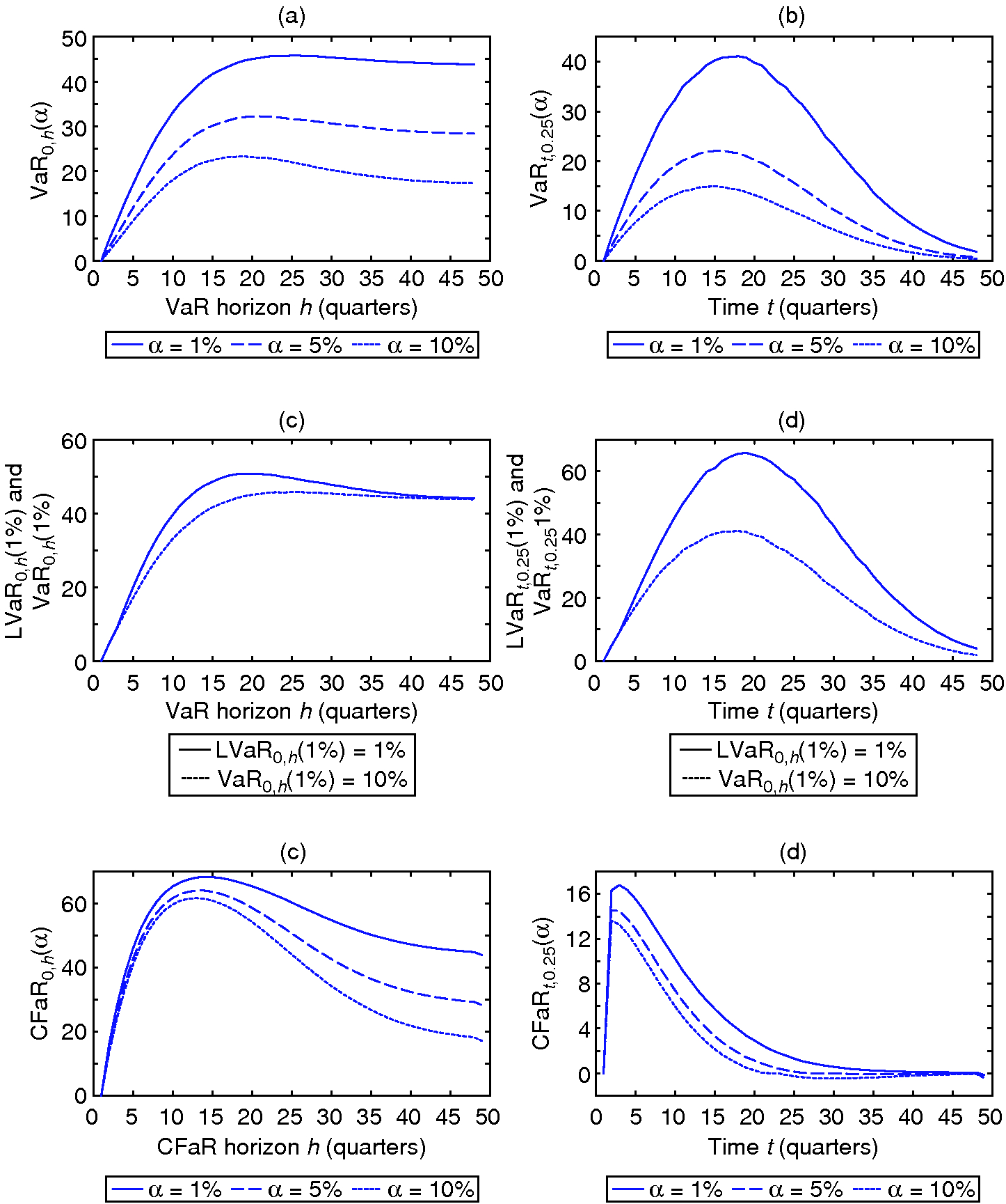
Figure 2: Risk dynamics over the fund life cycle. (a) VaR at fund initiation, ${\text{VaR}}_{\text{0},h}(\alpha )$, plotted as a function of the time horizon, $h$. (b) Quarterly VaR, ${\text{VaR}}_{t,\text{0.25}}(\alpha )$, plotted as a function of time $t$. (c) ${\text{LVaR}}_{\text{0},h}(\alpha )$ and ${\text{VaR}}_{\text{0},h}(\alpha )$ plotted as functions of the time horizon, $h$, for $\alpha =\text{1}$%. (d) ${\text{LVaR}}_{t,\text{0.25}}(\alpha )$ and ${\text{VaR}}_{t,\text{0.25}}(\alpha )$ plotted as functions of time $t$ for $\alpha =\text{1}$%. (e) CFaR at fund initiation, ${\text{CFaR}}_{\text{0},h}(\alpha )$, plotted as a function of the time horizon, $h$. (f) Quarterly CFaR, ${\text{CFaR}}_{t,\text{0.25}}(\alpha )$, plotted as a function of time $t$.

Figure 1 illustrates the dynamics of the cumulated capital drawdowns, capital distributions, net fund cashflows and fund value. It is important to acknowledge that the basic patterns of the model graphs shown in the figure conform to reasonable expectations of private equity fund behavior. In particular, the cashflow streams the model generates naturally exhibit a lag between the capital drawdowns and distributions, reproducing the typical development cycle of a fund and leading to the characteristic J-shaped private equity curve for the cumulated net fund cashflows that can be observed in Figure 1(c). In addition, note that the value dynamics of the fund shown in Figure 1(d) are also in line with expectations. Specifically, the value of the fund increases over time as the investment portfolio is built up, and decreases toward the end as increasingly fewer investments are left to be harvested. The model also captures the erratic nature of real-world private equity fund cashflows and value dynamics, which is indicated in Figure 1 by the 80% confidence intervals (dashed lines). Further, it is important to stress that the model is flexible enough to generate the potentially many different patterns of capital drawdowns and distributions. By altering the main model parameters, both the timing and magnitude of the fund cashflows can be controlled.

5.3 Value-at-risk dynamics

Parts (a) and (b) of Figure 2 illustrate the simulated VaR dynamics. Part (a) shows how the VaR at fund initiation (ie, at $t=0$), ${\mathrm{VaR}}_{0,h}(\alpha )$, changes with the time horizon, $h$. This reveals interesting patterns. For any given confidence level (10%, 5% and 1%), as the time horizon, $h$, increases, ${\mathrm{VaR}}_{0,h}(\alpha )$ initially rises sharply but then peaks and turns slightly downward. The initial sharp increase is in line with expectations. As the fund gradually draws down capital and builds up the investment portfolio, the investor’s risk exposure, and thus their maximum possible loss that can occur at some given confidence level, increases markedly. The slight decrease in VaR for long horizons $h$ is due to compounding effects in fund returns, which reduce the probability of large losses over long time horizons. The reduction in VaR is small, however, because intermediate capital distributions limit compounding effects in fund returns. The behavior of the VaR also depends on the chosen confidence level: for high confidence levels, ${\mathrm{VaR}}_{0,h}(\alpha )$ peaks more quickly and then falls more pronouncedly; for low confidence levels, ${\mathrm{VaR}}_{0,h}(\alpha )$ peaks more slowly and then stays near its maximum level. Note that the maximum value of ${\mathrm{VaR}}_{0,h}(\alpha )$ is well below the investor’s initial capital commitment of 100 for all the confidence levels considered. Thus, the maximum possible loss of a private equity fund investment is typically much lower than the investor’s total capital commitment.

Figure 2(b) further illustrates the VaR dynamics over the fund lifetime for a fixed time horizon of three months, ie, $h=0.25$. As expected, the fixed-horizon VaR of the fund investment, ${\mathrm{VaR}}_{t,0.25}(\alpha )$, increases as the fund draws down capital and peaks around the maximum average fund value (see also Figure 1). After the maximum level has been reached, ${\mathrm{VaR}}_{t,0.25}(\alpha )$ decays rapidly toward zero as capital distributions of the fund stepwise decrease the investor’s risk exposure. This basic pattern can be observed for all confidence levels considered. However, the results also show here that ${\mathrm{VaR}}_{t,0.25}(\alpha )$ peaks more quickly for lower levels of $\alpha$.

Overall, the dynamics illustrated in parts (a) and (b) of Figure 2 underline that there are specific private equity patterns in VaR dynamics that a sensible risk management framework must take into account. These patterns are a direct result of the complex cashflow structures of private equity fund investments, which lead to a situation where the mix of capital invested in the fund and cash holdings changes dynamically over the fund’s lifetime. In contrast, standard VaR implementations typically assume a static setting, where the mix in a position is unchanged over the time horizon of the VaR. To make these differences more obvious, Table 2 compares the VaR at fund initiation for a private equity fund investment and a mutual fund investment for different $h$. In order to make both fund investments comparable, it is assumed that the size of investment in the mutual funds equals the capital commitment to the private equity fund, $C_0=100$, and that the mutual and private equity funds have the same alpha, beta and idiosyncratic volatility.⁷⁷Note that the mutual fund is modeled by assuming that the value dynamics can be described by a standard geometric Brownian motion. The model parameters used for the private equity fund are again as given in Table 1. The results in Table 2 show several important differences. First, since a private equity fund is never fully invested in, due to intermediate capital distributions, the VaR of a mutual fund investment is higher than that of a private equity fund investment for all time horizons considered. Thus, when applied to private equity fund investments, standard VaR calculations can lead to biased conclusions about the investor’s true risk exposure. Second, the VaR of a private equity investment is very low for short time horizons because private equity funds involve stepwise capital drawdowns, and there is a more pronounced decrease in the VaR for long time horizons due to intermediate capital distributions.

Table 2: VaR comparison between a private equity fund and a mutual fund. [This table compares the VaR at fund initiation for a private equity fund investment and a mutual fund investment for different time horizons, $h$. In order to make both fund investments comparable, it is assumed that the size of investment in the mutual funds equals the capital commitment to the private equity fund, $C_{\text{0}}=\text{100}$, and that the mutual and private equity funds have the same alpha, beta and idiosyncratic volatility.Model parameters used for the private equity fund are as given in Table 1.]

	Mutual fund			Private equity fund
$?$	${\text{???}}_{\text{?}\mathbf{,}?}\mathbf{(}\text{?}\mathbf{\%}\mathbf{)}$	${\text{???}}_{\text{?}\mathbf{,}?}\mathbf{(}\text{?}\mathbf{\%}\mathbf{)}$	${\text{???}}_{\text{?}\mathbf{,}?}\mathbf{(}\text{??}\mathbf{\%}\mathbf{)}$	${\text{???}}_{\text{?}\mathbf{,}?}\mathbf{(}\text{?}\mathbf{\%}\mathbf{)}$	${\text{???}}_{\text{?}\mathbf{,}?}\mathbf{(}\text{?}\mathbf{\%}\mathbf{)}$	${\text{???}}_{\text{?}\mathbf{,}?}\mathbf{(}\text{??}\mathbf{\%}\mathbf{)}$
01	57.11	42.06	32.47	08.83	05.88	04.36
02	70.01	53.38	42.01	24.43	17.16	12.97
03	76.23	59.47	47.21	35.30	25.43	18.02
04	79.82	63.23	50.54	41.65	30.74	22.41
05	82.68	65.66	52.14	44.68	32.06	23.22
06	84.34	68.03	53.09	45.74	32.07	22.64
07	85.82	69.75	54.39	45.65	31.34	21.30
08	86.98	70.63	55.04	45.22	30.43	19.95
09	88.03	71.51	54.73	44.72	29.65	18.92
10	88.49	72.05	54.57	44.28	29.04	18.10
11	89.04	72.83	54.44	44.04	28.63	17.62
12	89.97	73.00	54.31	43.86	28.40	17.35

5.4 Liquidity-adjusted value-at-risk dynamics

Parts (c) and (d) of Figure 2 compare the standard VaR with the LVaR obtained by correcting fund values for potential secondary market discounts. The confidence level used for this comparison is 1%. As expected, the results highlight that illiquidity increases the investor’s risk exposure. In this sense, Figure 2(c) shows that the $\mathrm{LVaR}$ at fund initiation, ${\mathrm{LVaR}}_{0,h}(\alpha )$, is typically higher than the standard ${\mathrm{VaR}}_{0,h}(\alpha )$. However, the figure also shows that illiquidity only increases the investor’s risk exposure if the time horizon, $h$, under consideration is smaller than the funds’s total legal lifetime, $T_{\mathrm{l}}$, as ${\mathrm{LVaR}}_{0,T_{\mathrm{l}}}(\alpha )={\mathrm{VaR}}_{0,T_{\mathrm{l}}}(\alpha )$. The economic rationale behind this result is straightforward. Because a private equity fund is fully liquidated at the end of its legal lifetime, liquidity risk is fully resolved at $T_{\mathrm{l}}$. Thus, liquidity risk is only of importance if there is a mismatch between the investor’s expected holding horizon, $h$, and a fund’s legal lifetime. Consequently, for long-term investors with sufficient cash reserves, liquidity risk is only of minor importance.

The dynamics of the three-month LVaR, ${\mathrm{LVaR}}_{t,0.25}(\alpha )$, displayed in Figure 2(d) further highlight that the effects of illiquidity on the investor’s risk exposure over the life of the fund can be substantial. For the given confidence level of 1%, the maximum loss that can occur over a period of three months increases from around 41 to 66. Thus, for investors who face the risk of surprise liquidity shocks and need to sell their private equity positions on the secondary markets, ignoring liquidity risk can lead to substantially underestimated risk exposures.

5.5 Cashflow-at-risk dynamics

The dynamics of the developed CFaR measure are illustrated in parts (e) and (f) of Figure 2. The results highlight that an investor is exposed to substantial funding (or cashflow) risk when investing in private equity funds. Similarly to the above, Figure 2(e) shows how the CFaR at fund initiation, ${\mathrm{CFaR}}_{0,h}(\alpha )$, changes with the time horizon, $h$. In line with expectation, ${\mathrm{CFaR}}_{0,h}(\alpha )$ increases quickly during the commitment period, when the fund starts to draw down capital, and reaches a maximum after around twelve to fifteen quarters, depending on the $\alpha$ chosen. It is important to note that the maximum level is below the investor’s initial capital commitment, $C_0=100$, for all confidence levels considered. This is because private equity funds typically start to distribute capital before the committed capital has actually been fully drawn. Thus, investors typically do not need to reserve all their committed capital in cash, as distributions from existing investments can be used to partially finance open commitments. After the maximum level is attained, ${\mathrm{CFaR}}_{0,h}(\alpha )$ decreases because the capital distributions of the fund gradually increase the investor’s cash position. It is also interesting to see how the behavior of ${\mathrm{CFaR}}_{0,h}(\alpha )$ changes with the $\alpha$ chosen. For short time horizons, the differences between the curves for different levels of $\alpha$ are small, but these become larger as $h$ tends toward the fund lifetime, $T_{\mathrm{l}}$. The rationale behind this result is that capital distributions involve higher levels of uncertainty than capital drawdowns.

The fixed horizon $\mathrm{CFaR}$ for $h=0.25$ shown in Figure 2(f) further illustrates how cashflow risk changes with the development stage of the fund. In the early stages of a fund’s life, when it starts to call capital from the investors, ${\mathrm{CFaR}}_{t,0.25}(\alpha )$ is large and gives a measure of funding risk, ie, the maximum amount of cash the investor must hold in reserve over the next quarter in order to be able to meet capital calls. Later in a fund’s life, when it starts to gradually exit its portfolio companies and returns the proceeds to the investors, ${\mathrm{CFaR}}_{t,h}(\alpha )$ decreases and gives a measure of distribution risk, ie, the negative value of ${\mathrm{CFaR}}_{t,h}(\alpha )$ gives an indication of the minimum amount of cash distributed by the private equity fund over the next quarter.

5.6 Sensitivity analysis

In the environment of high uncertainty that characterizes private equity, there are limits to the predictive value of model parameters calibrated from historical data. It is therefore meaningful to evaluate and quantify the impact of parameter shocks that could materially change risk projections. Figures 3 and 4 illustrate a number of such shocks that should be applied for stress testing.

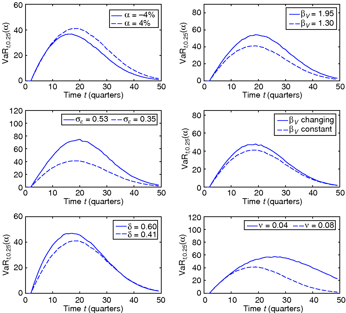
Figure 3: Sensitivity analysis VaR: dashed lines show the baseline case and solid lines highlight the effect of parameter changes; the confidence level used is $\alpha =\text{1}$%.

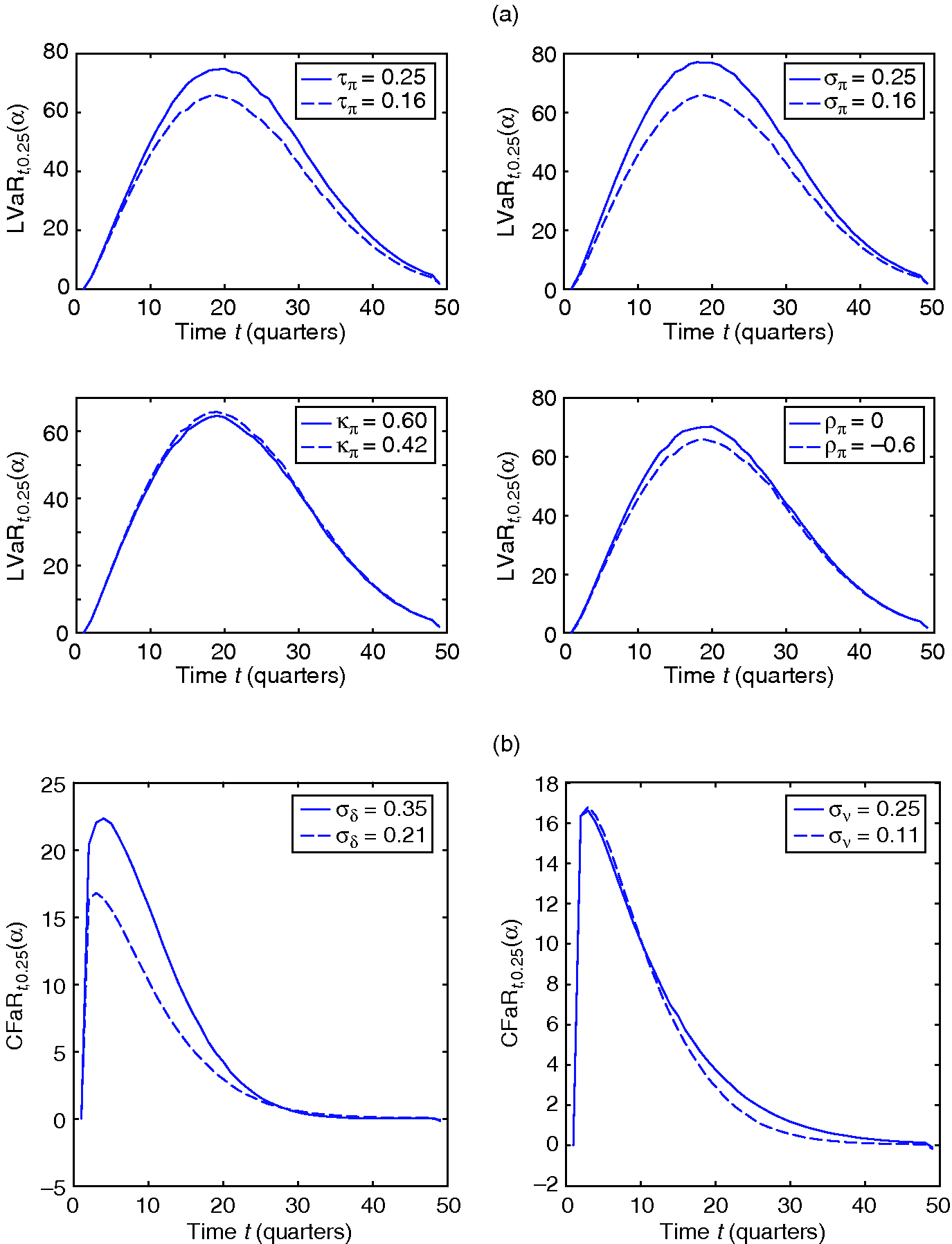
Figure 4: Sensitivity analysis for (a) LVaR and (b) CFaR: dashed lines show the baseline case and solid lines highlight the effect of parameter changes; the confidence level used is $\alpha =\text{1}$%.

Figure 3 identifies the main drivers of VaR. The previous numerical analysis used a strictly positive annual alpha of 4% for buyout funds. However, there are studies that find no evidence of positive alphas for buyout funds (see, for example, Driessen et al 2012). The figure shows that a lower annual alpha, of $-4$%, leads to a lower fixed-horizon VaR later in a fund’s life. The key risk parameters in the model are the market beta of a fund, ${\beta }_V$, and its idiosyncratic volatility, ${\sigma }_{\epsilon }$. In line with expectation, the figure shows that an increase in these two risk parameters, proxied here by multiplying both parameters by 1.5, leads to a substantial increase in the fixed-horizon VaR. Figure 3 further explores the effects of an important model extension on the VaR dynamics. Buyout transactions typically involve high leverage ratios early on, which are gradually reduced over the lifetime of the investment. Regarding the degree of financial leverage, Groh and Gottschalg (2009) report an average debt-to-equity ratio of around 3.0 at deal closing and an average debt-to-equity ratio of around 1.3 at deal exit. By definition, the leveraged (or equity) beta of an average stock market investment equals 1, and, with a typical debt-to-equity ratio of 0.5, the unleveraged (or asset) beta is 0.66. Assuming here that buyout investments have average unleveraged betas that are similar to those of publicly traded stocks, a corporate tax rate of 30% and a debt beta of 0.1 (see Kaplan and Stein 1990), a simple Modigliani–Miller calculation yields a leveraged beta of 1.84 at deal closing and of 1.17 at deal exit. In order to explore the effects of the changing deal leverage on the VaR dynamics, it is assumed that the beta of the fund decreases linearly from 1.84 to 1.17 over the fund lifetime. The effects of this model extension on the quarterly VaR are also illustrated in Figure 3. The results show that a decreasing beta leads to a higher fixed-horizon VaR compared with the baseline constant beta case. However, the effect is relatively small.

Moreover, the VaR dynamics also depend on the drawdown and distribution rate parameters. The figure shows that a higher mean drawdown rate, $\delta$, results in a faster investment pace and therefore leads to a faster increase in VaR in the early stages of a fund’s life and higher maximum VaR levels. The effect of a decrease in the mean distribution rate, $\nu$, which may occur during an economic downturn when exit opportunities for private equity funds deteriorate, is to increase VaR, particularly in the later phases of a fund’s life. This holds because a lower $\nu$ leads to a longer average investment duration, which increases the investor’s risk exposure.

In addition to these model parameters, the LVaR measure is also driven by the dynamics of secondary market discounts. Figure 4(a) shows that a higher long-run mean discount rate, ${\theta }_{\pi }$, and a higher volatility, ${\sigma }_{\pi }$, increase the fixed horizon LVaR. The effect of a higher mean-reversion rate, ${\kappa }_{\pi }$, is to slightly decrease LVaR, which holds because a high mean-reversion rate partly dampens volatility. In addition, increasing the correlation, ${\rho }_{\pi }$, of the discount rate with stock market returns increases LVaR, because it leads to a situation where high fund values coincide with high discount rates.

Figure 4(b) highlights the main drivers of the developed CFaR measure. The results indicate that a higher volatility, ${\sigma }_{\delta }$, of the drawdown rate increases funding risk at the start of a fund, whereas a higher volatility of the distribution rate increases the uncertainty about cashflows in the later stages of the fund’s life.

6 Extension to private equity fund portfolios

The previous analysis considered only investments in a single fund. In the following, the analysis is extended to a portfolio context. Since the VaR lacks subadditivity, this requires modeling portfolios of private equity funds explicitly. This section considers a static portfolio and a dynamic portfolio of funds.

6.1 Static portfolio of funds

Suppose that the portfolio of funds is formed of $n$ individual private equity funds. We first consider a so-called static portfolio of funds. In this case, the initial capital commitment, $C_0^{(i)}$, to each fund $i=1,\mathrm{\dots },n$ is set at the constitution of the portfolio and remains unchanged thereafter. The total value of the portfolio of funds is given by $V_t={\sum }_{i=1}^n{V}_t^{(i)}$. For simplicity, it is assumed here that all funds start at $t=0$ and have the same commitment period, $T_{\mathrm{c}}$, and the same total legal lifetime, $T_{\mathrm{l}}$. However, the funds in the model can have different risk and return characteristics as well as different drawdown and repayment dynamics. A complete model of the portfolio of funds is then given by the following system of SDEs for all $1\le i\le n$:

	$\mathrm{d}{V}_t^{(i)}$	$=V_t^{(i)}({\mu }_V^{(i)}\mathrm{d}t+{\beta }_V^{(i)}{\sigma }_M\mathrm{d}{B}_{M,t}+{\sigma }_{\epsilon }^{(i)}\mathrm{d}{B}_{\epsilon ,t}^{(i)})+\mathrm{d}{D}_t^{(i)}-\mathrm{d}{R}_t^{(i)},$		(6.1)
	$\mathrm{d}{D}_t^{(i)}$	$={\delta }_t^{(i)}(C_0^{(i)}-D_t^{(i)})\mathrm{d}t,{\delta }_t^{(i)}={\delta }^{(i)}+{\sigma }_{\delta }^{(i)}{B}_{\delta ,t}^{(i)},$		(6.2)
	$\mathrm{d}{R}_t^{(i)}$	$={\nu }_t^{(i)}{V}_t^{(i)}\mathrm{d}t,{\nu }_t^{(i)}={\nu }^{(i)}t+{\sigma }_{\nu }^{(i)}{B}_{\nu ,t}^{(i)},$		(6.3)

where it is assumed that

	$$\mathrm{d}{B}_{M,t}\mathrm{d}{B}_{\epsilon ,t}^{(i)}=0,\mathrm{d}{B}_{\delta ,t}^{(i)}\mathrm{d}{B}_{M,t}={\rho }_{\delta }^{(i)}\mathrm{d}t,\mathrm{d}{B}_{\delta ,t}^{(i)}\mathrm{d}{B}_{\epsilon ,t}^{(i)}=0,$$
	$$\mathrm{d}{B}_{\nu ,t}^{(i)}\mathrm{d}{B}_{M,t}={\rho }_{\nu }^{(i)}\mathrm{d}t\mathit{\hspace{1em}}\text{and}\mathit{\hspace{1em}}\mathrm{d}{B}_{\nu ,t}^{(i)}\mathrm{d}{B}_{\epsilon ,t}^{(i)}=0$$

for all $i=1,\mathrm{\dots },n$. In addition, note that the correlation between the drawdown rate dynamics of two funds $i$ and $j$ ($i\ne j$) is given in the model by ${\rho }_{\delta }^{(ij)}={\rho }_{\delta }^{(i)}{\rho }_{\delta }^{(j)}$ and the correlation between the distribution rate dynamics of two funds $i$ and $j$ ($i\ne j$) is given by ${\rho }_{\nu }^{(ij)}={\rho }_{\nu }^{(i)}{\rho }_{\nu }^{(j)}$. These two coefficients are also important risk management parameters. In particular, the average correlations across all funds in the portfolio control diversification in drawdowns and distributions: the smaller the average correlations, the greater the diversification in the drawdown and repayment policies, which ensures more regular cashflows; conversely, the larger the average correlations, the poorer the diversification, which can lead to more irregular portfolio cashflows.

6.2 Dynamic portfolio of funds

In order to develop a dynamic portfolio strategy for private equity fund investments, assume that the investor makes capital commitments to new funds at some frequency $\mathrm{\Delta }t$ (eg, quarterly). For simplicity, it is assumed that the investor can only commit capital to a single fund at each of the equidistant points in time: fund $i=1$ starts at time $t=0$, fund $i=2$ starts at time $\mathrm{\Delta }t$, and so on; fund $i=k$ starts at time $t=(k-1)\mathrm{\Delta }t$. For each fund $i$, the investor can dynamically choose the size of the capital commitment, $C_0^{(i)}$. Consistent with the literature on private equity commitment strategies (see, for example, Nevins et al 2004; de Zwart et al 2012), it is assumed in the following that the investor wants to attain a constant amount of capital invested in private equity funds over time. This can be achieved in the model by deriving a dynamic commitment strategy such that the squared difference between the constant target investment level, $\widehat{V}$, and the conditional expectation of the model portfolio value is minimized at each instant of time:

$$\underset{C_0^{(k)}}{\min }{(\widehat{V}-E[V_{k\mathrm{\Delta }t}\mid {ℱ}_{(k-1)\mathrm{\Delta }t}])}^2.$$

(6.4)

Using discrete-time versions of the processes (6.1)–(6.3), the conditional expectation contained in (6.4) can be stated as

	$E[V_{k\mathrm{\Delta }t}\mid {ℱ}_{(k-1)\mathrm{\Delta }t}]$	$={\displaystyle \sum _{i=1}^{k-1}}{V}_{(k-1)\mathrm{\Delta }t}^{(i)}(1+{\mu }_V^{(i)})\mathrm{\Delta }t+{\displaystyle \sum _{i=1}^{k-1}}{\delta }^{(i)}(C_0^{(i)}-D_{(k-1)\mathrm{\Delta }t}^{(i)})\mathrm{\Delta }t$
		$\mathrm{\hspace{1em}\hspace{1em}}-{\displaystyle \sum _{i=1}^{k-1}}{\nu }^{(i)}[k\mathrm{\Delta }t-(i-1)\mathrm{\Delta }t]V_{(k-1)\mathrm{\Delta }t}^{(i)}\mathrm{\Delta }t+{\delta }^{(k)}{C}_0^{(k)}\mathrm{\Delta }t.$		(6.5)

The first three terms on the right-hand side of (6.2) equal the expected portfolio value of all fund investments that are already in place, denoted by $V_{k\mathrm{\Delta }t}^{\ast }$ in the following. The fourth term equals the expected change in portfolio value due to the new capital commitment to fund $k$. Using the discrete-time approximation (6.2), the optimal commitment to fund $k$, $C_0^{(k)}$, can be derived by taking the derivatives of the objective function (6.4). This yields

$$C_0^{(k)}=\max \{\frac{\widehat{V}-V_{k\mathrm{\Delta }t}^{\ast }}{{\delta }^{(k)}\mathrm{\Delta }t},0\},$$

(6.6)

where taking the maximum here makes sure that the optimal commitment $C_0^{(k)}$ cannot get negative. The interpretation of (6.6) is straightforward. The investor will make new commitments to fund $k$ if the expected portfolio value of the fund investments already in place falls short of the target $\widehat{V}$, and will not make new commitments if it exceeds the target level. Overall, this gives a novel dynamic commitment strategy that is simple to implement. As shown in the numerical analysis below, this dynamic commitment strategy also has the attractive feature that it results in a constant fixed-horizon VaR over time.

6.3 Numerical results

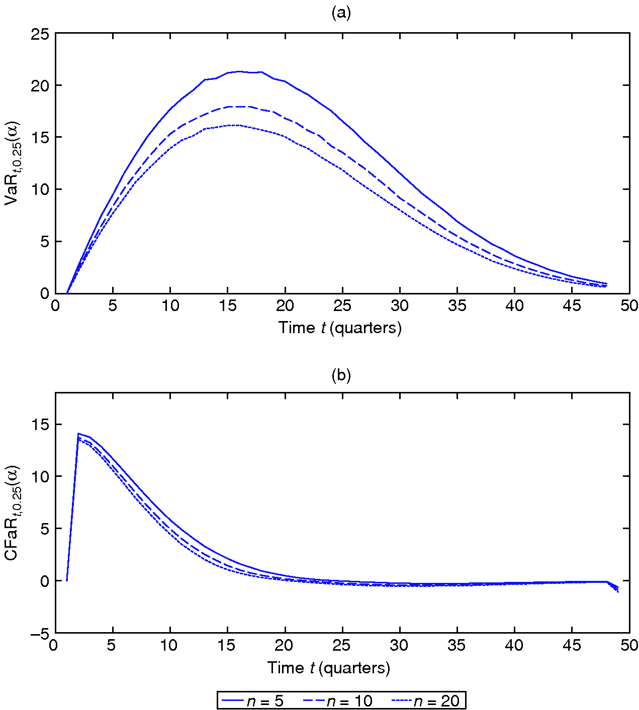
Figure 5: (a) VaR and (b) CFaR dynamics of a static portfolio of private equity funds for different portfolio sizes, $n$; the confidence level used is $\alpha =\text{1}$%. 

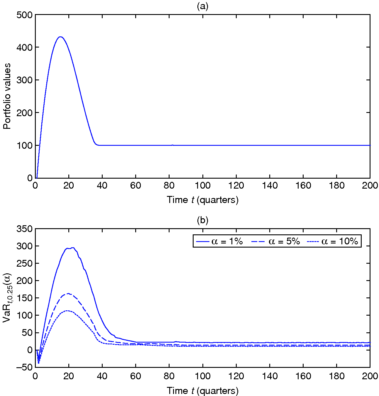
Figure 6: (a) Portfolio values and (b) VaR dynamics of a dynamic portfolio of private equity funds.

The subsequent numerical results are also derived using Monte Carlo simulations of the discrete-time processes given in Section 4.1. For the purpose of model illustration, it is assumed in the following that all funds in the portfolio have the same model parameters, which are again as given in Table 1. 

To illustrate the risk measures for a static portfolio of funds, assume that the investor’s total capital commitment equals $C_0=100$ and is equally split among the $n$ funds in the portfolio. Figure 5(a) illustrates the static portfolio VaR dynamics over the fund lifetime for a fixed time horizon of three months. The VaR dynamics are calculated for a confidence level of $\alpha =1$% and are shown for different portfolio sizes, $n$. As expected, the different graphs show the same time pattern as the single fund VaR dynamics illustrated in Figure 2(b). This behavior is due to the fact that we assume that all funds start at $t=0$ and have the same legal lifetime of $T_{\mathrm{l}}=12$ years. The figure also shows that portfolio diversification reduces the VaR, since the value dynamics of the funds in the portfolio are not perfectly correlated. As expected, this reduction in risk increases with $n$. In addition, the fixed horizon static portfolio CFaR for $h=0.25$ shown in Figure 5(b) illustrates how cashflow risk changes with the size, $n$, of the portfolio. Similar to the VaR, the results reveal that cashflow risk is slightly reduced by diversification, since the capital drawdowns (and capital distributions) of the portfolio funds are also not perfectly correlated in the model.

Finally, the novel dynamic commitment strategy is illustrated in Figure 6. The dynamics of the mean portfolio values shown in part (a) reveal that the developed commitment strategy does (on average) lead to the correct target allocation to private equity funds, since the mean portfolio value converges to the target level of $\widehat{V}=100$ over time. The dynamics shown in Figure 6(a) further reveal that the convergence to the target portfolio value can require significant amounts of time when an investor has to build up a private equity portfolio from scratch. In the simulation, it takes around thirty-eight quarters or 9.5 years for the mean portfolio value to get close to the target value. In addition, the figure implies that building up a private equity portfolio typically requires some degree of so-called overcommitment, where early commitments exceed the target exposure. This overcommitment increases the speed of convergence to the target exposure but has the drawback that the mean portfolio value initially overshoots the target level. This finding is consistent with the results of other studies which also show that building up a private equity fund portfolio requires some degree of initial overcommitment (see, for example, de Zwart et al 2012). Figure 6(b) further illustrates the portfolio VaR dynamics over time for a fixed horizon of three months. The results show that the fixed-horizon VaR also converges to a constant level over time. Hence, the investor can attain a constant risk exposure under the developed dynamic commitment strategy.

7 Conclusion

Although risk management has been a well-studied field in financial modeling for over three decades, our understanding of how to correctly quantify and manage the risks of investing in private equity remains limited. Because of institutional features that complicate the use of standard risk management tools, most investors still employ relatively simplistic approaches to measure the risks of investing in private equity. However, with growing exposure to private equity, it has become more important to fully understand and correctly quantify the risks of investing in this asset class. Moreover, more sophisticated risk management will also be an essential catalyst for further growth of the asset class. Surprisingly, the academic literature has largely overlooked this fact; at present, we lack an adequate risk model for private equity that allows all relevant risks to be accurately addressed.

This paper aims to fill a gap in the literature by developing the first comprehensive risk management framework for private equity fund investments. The framework addresses the three main sources of risk that private equity investors face when investing in this asset class: market risk, liquidity risk and cashflow risk. Underlying the framework is a stochastic model for the value and cashflow dynamics of private equity funds, which allowed us to derive three dynamic risk measures for private equity fund investments: VaR, LVaR and CFaR. We calibrated the model to data from buyout funds and illustrated the dynamics of the risk measures using Monte Carlo simulations. A model extension also studied the dynamics of the risk measures for portfolios of funds and developed a novel dynamic commitment strategy for private equity funds that enables investors to attain a constant fixed-horizon VaR.

Declaration of interest

The author reports no conflicts of interest. The author alone is responsible for the content and writing of the paper.

Acknowledgements

I thank Farid AitSahlia (the editor), Attilio Meucci, Dale W. R. Rosenthal and an anonymous referee for helpful comments and discussions. Earlier versions of the paper benefited from comments by participants at the NUS–RMI Ninth Annual Risk Management Conference in Singapore.

References

Ang, A., Chen, B., Goetzmann, W. N., and Phalippou, L. (2013). Estimating private equity returns from limited partner cash flows. Working Paper, Social Science Research Network (http://doi.org/b78n).

Bongaerts, D., and Charlier, E. (2009). Private equity and regulatory capital. Journal of Banking and Finance 33(7), 1211–1220 (http://doi.org/bksnrs).

Cochrane, J. H. (2005). The risk and return of venture capital. Journal of Financial Economics 75(1), 3–52 (http://doi.org/c9hczj).

de Zwart, G., Frieser, B., and D. van Dijk (2012). Private equity recommitment strategies for institutional investors. Financial Analysts Journal 68(3), 81–99 (http://doi.org/b78p).

Diller, C., and Herger, I. (2008). Private equity: will you take the risk? Private Equity International, 106–109.

Driessen, J., Lin, T.-C., and Phalippou, L. (2012). A new method to estimate risk and return of non-traded assets from cash flows: the case of private equity funds. Journal of Financial and Quantitative Analysis 47(3), 511–535 (http://doi.org/b78q).

Ewens, M., Jones, C. M., and Rhodes-Kropf, M. (2013). The price of diversifiableable risk in venture capital and private equity. Review of Financial Studies 26(8), 1854–1889 (http://doi.org/b78r).

Groh, A., and Gottschalg, O. (2009). The opportunity cost of capital of US buyouts. Working Paper 14148, National Bureau of Economic Research (http://doi.org/bp47t8).

Harris, R. S., Jenkinson, T., and Kaplan, S. N. (2014). Private equity performance: what do we know? Journal of Finance 69(5), 1851–1882 (http://doi.org/b78s).

Hochberg, Y., Ljungqvist, A., and Vissing-Jorgensen, A. (2014). Informational hold-up and performance persistence in venture capital. Review of Financial Studies 27(1), 102–152 (http://doi.org/b78t).

Jorion, P. (2001). Value at Risk: The New Benchmark for Managing Financial Risk, 2nd edn. McGraw-Hill.

Kaplan, S. N., and Schoar, A. (2005). Private equity performance: returns, persistence and capital flows. Journal of Finance 60(4), 1791–1823 (http://doi.org/fpt6wr).

Kaplan, S. N., and Stein, J. C. (1990). How risky is the debt in highly leveraged transactions? Journal of Financial Economics 27(1), 215–245 (http://doi.org/d5zbfw).

Kleymenova, A., Talmor, E., and Vasvari, F. P. (2012). Liquidity in the secondaries private equity market. Working Paper, London Business School.

Kloeden, P. E., and Platen, E. (1999). Numerical Solution of Stochastic Differential Equations. Springer.

Korteweg, A., and Sorensen, M. (2010). Risk and return characteristics of venture capital-backed entrepreneurial companies. Review of Financial Studies 23(10), 3738–3772 (http://doi.org/d4s998).

Ljungqvist, A., Richardson, M., and Wolfenzon, D. (2008). The investment behavior of buyout funds: theory and evidence. Working Paper 14180, National Bureau of Economic Research (http://doi.org/cdj2h4).

Malherbe, E. (2004). Modeling private equity funds and private equity collateralised fund obligations. International Journal of Theoretical and Applied Finance 7(3), 193–230 (http://doi.org/bwzrsh).

Nevins, D., Conner, A., and McIntire, G. (2004). A portfolio management approach to determining private equity commitments. Journal of Alternative Investments 6(4), 32–46 (http://doi.org/cjsb45).

Phalippou, L., and Gottschalg, O. (2009). The performance of private equity funds. Review of Financial Studies 22(4), 1747–1776 (http://doi.org/fr93x9).

Robinson, D. T., and Sensoy, B. A. (2011). Cyclicality, performance measurement, and cash flow liquidity in private equity. Working Paper 17428, National Bureau of Economic Research (http://doi.org/czs6wh).

Serfling, R. J. (1980). Approximation Theorems of Mathematical Statistics. Wiley.

Sorensen, M., Wang, N., and Yang, J. (2014). Valuing private equity. Review of Financial Studies 27(7), 1977–2021 (http://doi.org/b78v).

Takahashi, D., and Alexander, S. (2002). Illiquid alternative asset fund modeling. Journal of Portfolio Management 28(2), 90–100 (http://doi.org/fs7z4q).

Download PDF Appendix 1

• Keywords
• Private equity
• Risk management
• Value-at-risk (VAR)
• Original research