Journal of Network Theory in Finance
ISSN:
2055-7809 (online)
Editor-in-chief: Ron Berndsen

Evaluating the role of risk networks in risk identification, classification and emergence
Need to know
- The authors introduce a novel methodology to generate risk networks, which relaxes some assumptions of past related work, including prominent work by the World Economic Forum.
- The risk network can serve as a robust risk classification framework, free from externally-imposed artificial constructs (e.g. risk classification based on regulatory requirements).
- By applying it to a UK (re)insurance dataset, the authors use the resulting risk network to evaluate the ‘horizon scanning’ capacity of every included firm.
- The risk network uncovers a general mismatch between independent and systemic impact of risks, with authors arguing that this mismatch can be used to classify certain risks as ‘emerging’.
Abstract
Modern society heavily relies on strongly connected socio-technical systems. As a result, distinct risks threatening the operation of individual systems can no longer be treated in isolation. Risk experts are actively seeking ways to relax the risk independence assumption that undermines typical risk management models. Prominent work has advocated the use of risk networks as a way forward. However, the inevitable biases introduced during the generation of these survey-based risk networks limit our ability to examine their topology and in turn challenge the utility of the very notion of a risk network. To alleviate these concerns, we propose an alternative methodology for generating weighted risk networks. We subsequently apply this methodology to an empirical data set of financial data. This paper reports our findings on the study of the topology of the resulting risk network. We observe a modular topology and reason on its use as a robust risk classification framework. Using these modules, we highlight a tendency of specialization during the risk identification process, with some firms being solely focused on a subset of the available risk classes. Finally, we consider the independent and systemic impact of some risks and attribute possible mismatches to their emerging nature.
Introduction
1 Introduction
An enhanced understanding of the nature of risk is the epitome of modern science (Bernstein 1996; Buchanan and O’Connell 2006), with its successful management yielding significant benefits across a wide range of societal facets (Ganin et al 2016; Helbing 2013; Vespignani 2012). In this context, risk is traditionally defined as the “effect of uncertainty on objectives”; it is generally quantified as the probability of an event materializing multiplied by its expected impact (International Organization for Standardization 2009). The objective of risk management is thus to mitigate events that can lead to an undesirable outcome (Pritchard 2014).
Underlying this objective is the assumption that each adverse event is independent, eg, interdependence bears no effect when quantifying risk (International Organization for Standardization 2009). Yet, the operation of modern society largely depends on precisely this interdependence (World Economic Forum 2017), as it supports the global exchange of “people, goods, money, information, and ideas” (Helbing 2013). Incorporating the effect of interdependence into the risk management process has attracted much recent interest (Battiston et al 2012; Battiston et al 2016a; DasGupta and Kaligounder 2014; Helbing 2013; Roukny et al 2013; Szymanski et al 2015), partly due to the 2007–8 global financial crisis and the way in which traditional risk models, also grounded in the assumption of risk independence, failed to foresee it (Battiston et al 2016a,b; Besley and Hennessy 2009; Schweitzer et al 2009).
One way of exploring the effect of risk interdependence is by considering how risks interact (Helbing 2013; Szymanski et al 2015). A prominent example of this approach can be found in the annual global risk report, generated by the World Economic Forum (WEF). Currently in its twelfth edition, this report explicitly explores the effect of risk interdependence by considering risk networks. Within each network, a risk (node) is connected, via weighted links, to a number of other risks. In this particular example, links are established through a survey of roughly 750 experts – from government, academia and industry – with participants being asked the following: “Global risks are not isolated and it is important to assess their interconnections. In your view, which are the most strongly connected global risks? Please select three to six pairs of global risks” (see World Economic Forum 2017, Appendix B).
This question focuses on describing the local structure of the risk network, and it is a variant of the so-called name generator: a tool often deployed by surveys that focus on constructing the overall structure of (mostly social) networks using ego networks (Bidart and Charbonneau 2011; Merluzzi and Burt 2013). Despite the wide deployment of these name generators (Merluzzi and Burt 2013), the resulting data must be approached with caution due to its inevitable exposure to multiple sources of contamination (Bearman and Parigi 2004; Bidart and Charbonneau 2011; Newman et al 2011). In the case of the WEF report, the derived risk network must be regarded with skepticism for at least two reasons. First, participants are explicitly given an upper and lower bound on the number of connections that they can utilize, inevitably biasing the overall connectivity of the risk network. Second, the nature of the link implied through the questionnaire is ambiguous, as a link between two risks may suggest (a) a causal link (ie, risk A causes risk B, and hence they are connected) or (b) a similarity link (ie, risk A is similar to risk B, and hence they are connected). This accumulating ambiguity can undermine the consequent analysis of the resulting risk network. For example, consider the most connected risk. If (a) is the case, then this risk is expected to play a key role in terms of triggering large-scale cascades, ie, it will be of high systemic importance (Albert and Barabási 2002). However, if (b) is the case, such heightened connectivity merely suggests that its neighboring risks are somewhat similar. The impact of this ambiguity becomes even harder to evaluate once sophisticated analysis is applied to such networks. For example, consider the recent work of Szymanski et al (2015), who have used the WEF risk network to analyze its failure dynamics. Despite the theoretical rigor of the analysis itself, its inevitable dependence on the network’s topology calls into question the eventual outcome of the analysis, since the ambiguity contained within the network itself is neither evaluated nor accounted for.
Working toward capturing risk interdependence in a more robust way, we developed a methodology to generate weighted risk networks based on risk similarity, where risks are connected based on the similarity of their characteristics. By applying this methodology to an empirical data set of 143 risks, each described using twenty-four unique tags, this paper discusses the role of risk interdependence in terms of three core components of the risk management process:
- (a)
risk classification, which is independent of externally imposed labels;
- (b)
evaluation of the horizon-scanning capacity of a given firm; and
- (c)
identification of emerging risks, based on the influence of interconnectivity on their independent impact, and how they underlie firm interactions.
2 Results
In what follows, we analyze the topology of the risk network, focusing particularly on its modular composition (see the supporting information (SI) in the online appendix for detailed visualizations). We then evaluate the capacity of each firm to identify risks uniformly across all observed modules; the ability to do so corresponds to an enhanced horizon-scanning capacity. Finally, we use a simple epidemic model (Gutfraind 2010; Pastor-Satorras et al 2015; Watts 2002) to evaluate the systemic importance of each risk in terms of its ability to trigger subsequent risks. By doing so, we compare the reported independent impact of each risk with its evident systemic one, attributing possible differences to their “emerging” natures. The consequent interaction between firms is briefly evaluated in the form of liability networks.
2.1 Emergence of risk modules
In the context of the risk network, our analysis identifies five distinct modules, composed of forty-seven (module 1), thirty-five (module 2), twenty-five (module 3), twenty-one (module 4) and sixteen (module 5) risks, respectively (see Figure 1). A module is defined as a group of nodes that are densely connected to each other but loosely connected with nodes that belong to different modules (Danon et al 2005; Fortunato 2010). In the context of the risk network, every module can be regarded as a distinct risk class, where its formation solely depends on the underlying characteristics of each risk (see Section 4). This bottom-up method is different to the top-down approach generally adopted in risk classification schemes, which builds on externally imposed labels based on a particular organizational function, eg, “strategic risk” (Kaplan and Mikes 2012), or a regulatory requirement, eg, “capital ratio” from the Basel III regulatory framework (Basel Committee on Banking Supervision 2010).
Increased levels of connectivity correspond to increased levels of risk similarity, in terms of both intraconnectivity (within a module) and interconnectivity (between modules). Consequently, if a given set of conditions triggers a particular risk, the same condition(s) will also affect (and potentially trigger) its neighboring nodes, depending on how similar they are in terms of their underlying characteristics (Allan et al 2013). With risk similarity in mind, consider the case of module 2: heightened intraconnectivity indicates that the risks contained within it are increasingly similar. Conversely, module 3 is defined by relatively low levels of intraconnectivity. Shifting focus to the interconnectivity aspect, heightened interconnectivity identifies related risk classes; the strong link between module 2, composed of regulatory risks, and Module 5, composed of political risks, serves as an intuitive example.

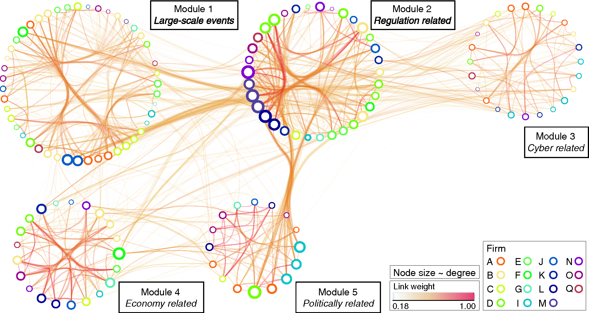
With respect to the actual composition of each module, it is of particular interest to identify risks that contradict the overall theme of each module. For example, module 3 is principally composed of cyber-related risks, evident from the word-decomposition of the risk labels found within the module (see the SI for Section 2 in the online appendix). Among these cyber-related risks, the risk “global population changes” is also present; this may seem to be a rather counterintuitive inclusion at first, but it is one deeply embedded within the technological realm of module 3. One can easily reason that health is highly dependent on the rate of technological advancement, which in turn affects the population size. However, in the case of traditional risk classification, “global population change” would have been grouped under a distinctly different label, eg, “insurance and demographic risk” (see Kelliher et al 2013), compared with the rest of the risks contained in module 3. More generally, these risk modules can uncover risks that are seemingly distinct in terms of their attributed labels – such as in the “global population changes” case – yet are increasingly similar in terms of their underlying characteristics. This in turn suggests some sort of similarity in how they might be mitigated.
2.2 Evaluation of horizon-scanning capacity
The risk management process can be summarized as a process designed to “identify to analyze to evaluate to treat” a particular risk (International Organization for Standardization 2009). With horizon scanning being the first step in this process, a firm capable of identifying risks across all risk classes limits its exposure to unidentified risks. By considering the basis on which the network is developed, this insight becomes intuitive: when a firm identifies, and eventually treats, a risk of a given class, the firm inevitably becomes somewhat shielded from the impact of similar risks, ie, risks that belong to the same class (World Economic Forum 2017). Conversely, the tendency of a firm to identify risks from particular risk classes biases its horizon-scanning function and in turn increases its overall risk exposure, especially if entire risk classes remain uncovered.
| Module | |||||
| Firm | 1 | 2 | 3 | 4 | 5 |
| A | 35.7 | 0.0 | 35.7 | 0.0 | 28.6 |
| B | 44.4 | 16.7 | 16.7 | 22.2 | 0.0 |
| C | 61.5 | 7.7 | 15.4 | 7.7 | 7.7 |
| D | 14.3 | 50.0 | 14.3 | 14.3 | 7.1 |
| E | 60.0 | 30.0 | 0.0 | 10.0 | 0.0 |
| F | 33.3 | 33.3 | 0.0 | 33.3 | 0.0 |
| G | 33.3 | 16.7 | 0.0 | 33.3 | 16.7 |
| I | 28.6 | 7.1 | 35.7 | 7.1 | 21.4 |
| J | 44.4 | 22.2 | 0.0 | 22.2 | 11.1 |
| K | 0.0 | 42.9 | 42.9 | 14.3 | 0.0 |
| L | 0.0 | 33.3 | 0.0 | 33.3 | 33.3 |
| M | 20.0 | 60.0 | 20.0 | 0.0 | 0.0 |
| N | 0.0 | 57.1 | 14.3 | 28.6 | 0.0 |
| O | 36.4 | 18.2 | 9.1 | 9.1 | 27.3 |
| Q | 33.3 | 33.3 | 16.7 | 16.7 | 0.0 |

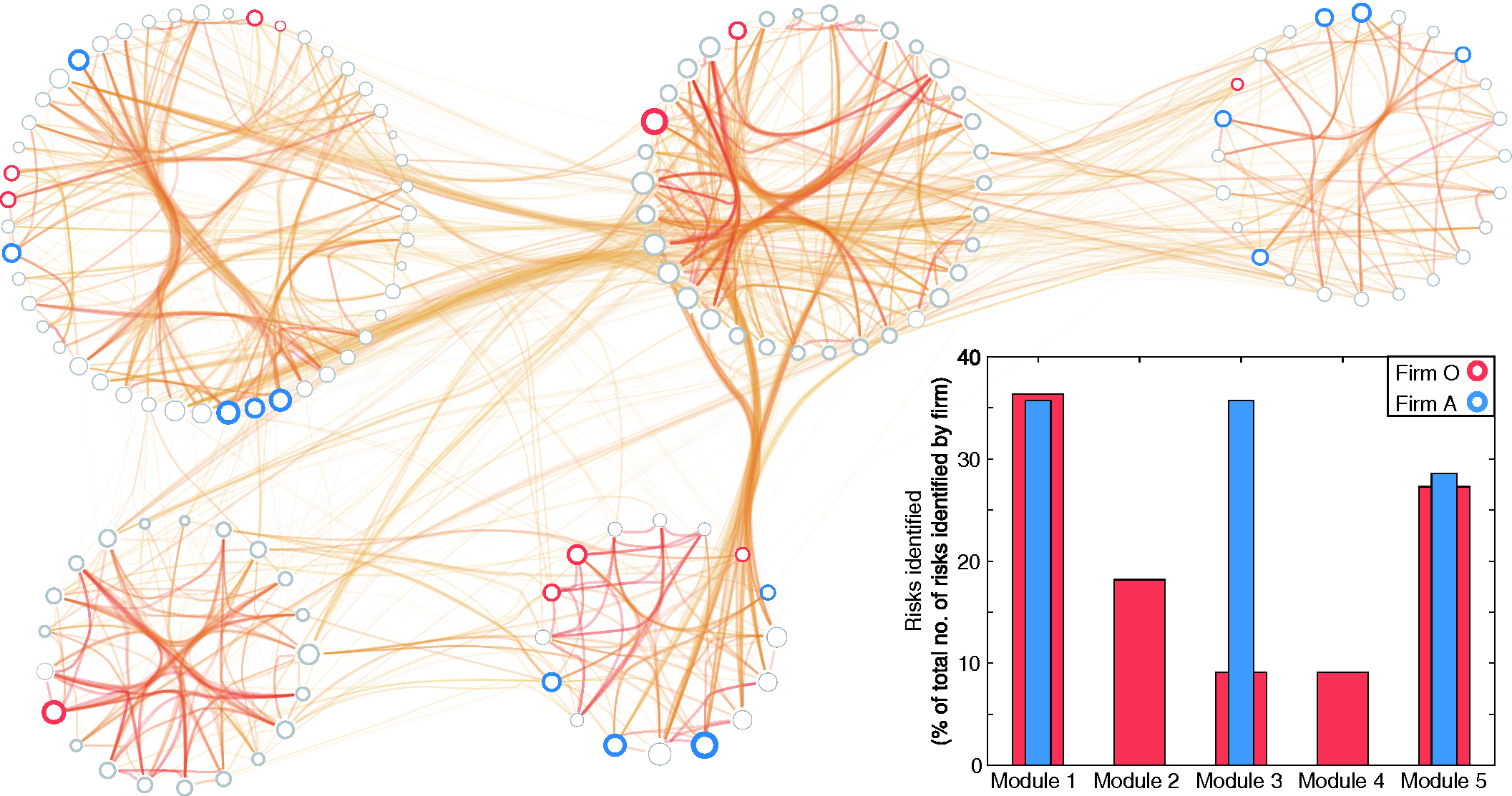
Table 1 details the horizon-scanning capacity of each firm, as reflected by the number of risks identified in each of the five risk classes (reported in the form of a percentage). An example of the aforementioned bias toward missing particular risk classes is firm A, with its horizon-scanning deployment specializing in the risks that belong to modules 1, 3 and 5 (see Figure 2, blue). As a result, firm A is unaware of the risks that belong to modules 2 and 4. Conversely, firm O is able to identify at least one risk across all five modules (see Figure 2, red), and hence it is well equipped to tackle risks that have remained unidentified but are contained within these five modules.
More generally, the majority of firms appear to specialize in the identification of risks that belong to particular risk classes. In other words, firms tend to tailor their horizon-scanning function toward the identification of risks of a particular nature (ie, risks that belong to the same module). Network-based techniques can highlight these instances and help mitigate them by broadening the focus of the corresponding horizon-scanning function.
2.3 Identifying emerging risks and who they affect
An emerging risk can be defined as “a material, previously unconsidered risk or changing risk factor that has the potential to significantly alter the firm’s risk profile” (ORIC International 2017). These risks are “developing or already known risks which are subject to uncertainty … and are therefore difficult to quantify using traditional risk assessment techniques” (International Actuarial Association 2008). In this context, we translate this uncertainty as the way in which interconnectivity affects the systemic impact of a risk in relation to its independent impact. In other words, an emerging risk is one whose position in the network alters its independent impact, either in a positive or negative way.
The independent impact of every risk considered herein is reported in a qualitative manner (ie, “high”, “medium” or “low”) by its respective firm, as set by the industry standard ISO 31000 (International Organization for Standardization 2009). The systemic impact is evaluated using a simple threshold model (Gutfraind 2010; Pastor-Satorras et al 2015; Watts 2002), which essentially models a cascade in which a risk materializes, and subsequently triggers related risks in a probabilistic manner, depending on the risk similarity of a risk pair (see Section 4). The final number of risks consequently affected by the initially affected risk corresponds to its systemic impact. As such, a risk whose materialization triggers a large number of subsequent risks is assigned a high systemic impact, and vice versa.
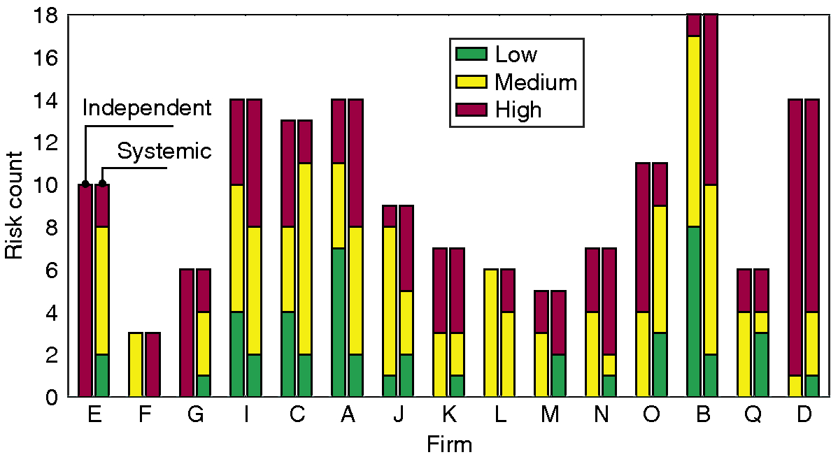
Overall, a general mismatch exists between the independent and systemic impact across the most influential risks, which indicates that the assumption of risk independence obscures the emerging nature of risks (Figure 3). This misalignment is consistent across most firms, highlighting an overall tendency to underestimate the increased systemic impact of particular risks. Consider Risk IDX 118 (European data protection rules), which has been assessed to have a “low” independent impact yet is of “high” systemic impact (it triggers an average of 32.9 subsequent risks and ranks fourth out of 143 risks; see Table 2). In other words, the assumption of risk independence conceals the systemic nature of these risks, and in turn shrouds its emerging nature.

| Trigger | Firm who | Systemic | ||
|---|---|---|---|---|
| risk | identified | impact | Independent | |
| IDX | Risk title | risk | (rank) | impact |
| 65 |
Political intervention (tax, caps, levies, rating factors, data, etc) |
J | High (1st) | Medium |
| 12 |
Brexit and Scottish independence |
F | High (2nd) | Medium |
| 107 |
Legal action driving changing claims patterns |
B | High (3rd) | Medium |
| 118 |
European data protection rules |
B | High (4th) | Low |
| 13 |
Mandate extension to commercial properties |
F | High (5th) | Medium |
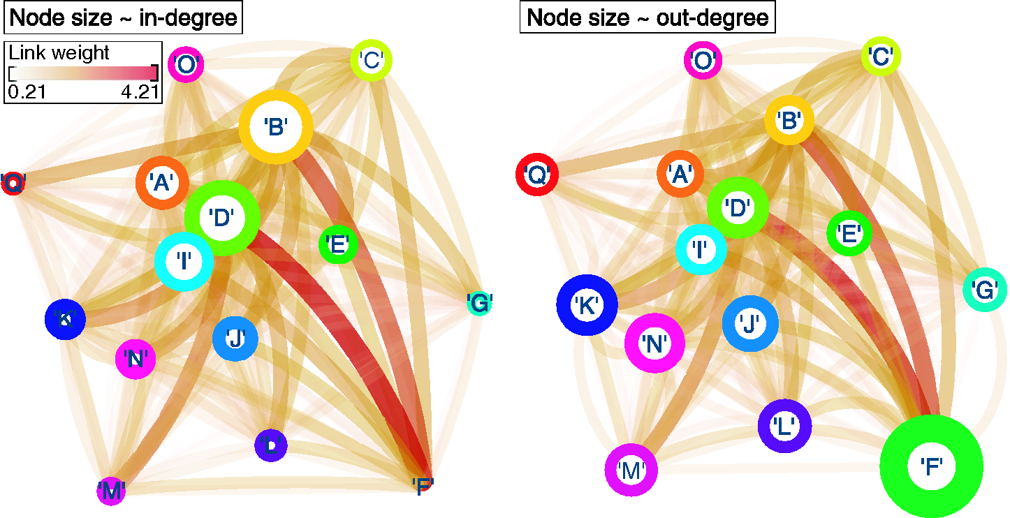
The consequent interaction between firms, as it emerges through the systemic nature of each risk, can be examined by considering the liability network. In this case, each node corresponds to a firm, and a link between firms and reflects the ability of at least one risk reported by firm to interact with at least one risk reported by firm . In addition, link weight corresponds to the number of times all risks reported by firm interact with risks reported by firm (Figure 4). This weight is normalized over the total number of risks reported by firm in order to account for the variability in the number of risks reported by each firm. Note that, despite the symmetry in link directionality, this normalization scheme allows for a link between firms and to be of a different weight compared with the link between firms and ; thus, we consider the liability network to be directed.
The liability network can be used to identify firms that are heavily exposed to the systemic impact of particular risks, and to highlight possible collaborations. For example, firm D is affected the most, as is evident by its having the largest weighted in-degree (proportional to node size; Figure 4(a)). In addition, the largest contribution comes from risks that have been reported by firm F. In other words, risks that have been reported by firm F are very similar to those reported by firm D and in turn are increasingly likely to affect the former (firm F). Similarly, risks reported by firm F have a high systemic impact (Figure 4(b)), making firm F a key collaborator from which information sharing can benefit affected firms, such as firm D. Therefore, one can envision a collaboration between firms F and D in an attempt to prevent risk more efficiently.

3 Discussion
In this paper, we have presented an evaluation of how risk interdependence affects the risk management process. In contrast to previous studies, which focus on survey-based risk networks, we have introduced an empirical-based, quantitative risk network. In this respect, we have focused on
- (a)
the emergence of network modules,
- (b)
the “horizon scanning” capacity of individual firms, and
- (c)
emergent risks and how they reflect firm interactions.
Modules within the risk network provide an intuitive way for classifying risk. Typically, risk classification takes place within the boundary of individual firms through the imposition of (what is hoped to be) meaningful labels. Each such label relates a particular aspect of a firm to its economic value, eg, “market risk” relates market movement to fluctuations in the value of existing assets, which in turn affects a firm’s liabilities and income. Yet such classification is driven by externally imposed labels, which can fuel ambiguity, resulting in similar risks being grouped differently. A recent report by the Institute and Faculty of Actuaries highlights this inconsistency by means of an example, where “one organization may class failure of a project as operation risk, while another class[es] it as strategy risk” (Kelliher et al 2013). Transitioning from high-level risks, such as the ones considered herein, to low-level risks fuels the frequency of such inconsistencies further, as the number of possible labels that can be attributed to any one risk explodes (Kelliher et al 2013).
In contrast, the methodology proposed herein provides an intuitive way for classifying risk. By looking beyond a risk’s label, the explicit focus on a risk’s underlying characteristics ensures that the classification process is not obscured by externally imposed labels. Rather, the focus is on risk similarity, ensuring that risks belonging to the same module are, in fact, alike. As a result, these modules can include risks that are similar in principle yet described by seemingly unrelated labels with respect to the rest of the module. Consequently, resources spent in managing risks that appear to be different but are fundamentally similar (ie, they belong to the same risk module) can be saved, effectively streamlining the risk management process.
By exploiting the emergence of these modules, a firm can navigate toward enhanced horizon-scanning capabilities by identifying a diverse set of risks, ie, across all identified network modules. Considering the similarity-based construction of the risk network, the ability to identify risks from each module suggests that even though a firm may have missed some risks, its overall preparedness is high, as the remaining risks within that module are similar in nature. Overall, our work shows that the majority of firms specialize in the identification of risks that are of similar nature (ie, risks that belong to the same “risk class”). While such specialization is understandable, it can also increase risk exposure due to unidentified risks creeping in. Introducing network-based techniques into the overall risk management process can help contain this effect, improving the overall effectiveness of the risk management process.
Finally, we consider the effect of interconnectivity in terms of a possible mismatch between the independent and systemic impact of any given risk. We refer to risks that exhibit this mismatch as emerging risks. Focusing on risks where interconnectivity has a worsening effect, we are able to identify risks with a small, independent impact that are yet capable of a larger systemic impact. Such insight can be used to minimize biases introduced by traditional tools, eg, risk registers (International Organization for Standardization 2009), where attention is skewed toward risks with a high independent impact. In doing so, the likelihood of omitting risks with a low independent impact yet potentially high systemic impact can be minimized. In addition, by translating the systemic impact of each risk into a liability network, we can identify beneficial collaborations between firms, where the neighbor of a firm can hold valuable information with respect to the risks that impact it (eg, firms D and F; Figure 4). In principle, one can envision such information being used to promote mutually beneficial collaborations that can increase risk mitigation efficiency.
With that in mind, it is worth highlighting that firms are complex, multifaceted systems operating across a wide range of environments (regulatory, commercial, etc). Therefore, the utility of the liability network in identifying joint exposures that emerge from this rich variety of dependencies depends on a priori information. Consider a simple example in which contractual dependencies have been analyzed, and the risk of heavy reliance to a particular partner has been identified. On the one hand, if this risk is appropriately recorded, then its contribution to the liability network will be present. On the other hand, if the risk has been omitted, then, inevitably, the liability network will be incomplete, and hence its utility will be diminished.
In conclusion, the use of quantitative risk networks can significantly contribute to spurring the discussion on the interdependent nature of risk and its effect. The ability to map risk interdependence in the form of network modules provides a natural way to classify risk, which in turn can provide an intuitive way to reduce the number of risks that can be managed from several hundred to a handful, focusing risk management efforts. With that in mind, strategies can be formulated to prevent the occurrence of multiple risks that belong to the same class, and therefore increase effectiveness and efficiency of the overall risk management process. In addition, the capacity to evaluate possible limitations in the horizon-scanning capacity of a firm can provide valuable insights into possible exposures, while the capacity to identify emerging risks contributes to the reduction of a firm’s exposure to large-scale, systemic failures.
4 Methods
4.1 Data
The risk data set has been obtained from ORIC International, an operational risk consortium for the (re)insurance and asset management sector (http://www.oricinternational.com). The data set contains 143 unique risks, as reported by fifteen firms active in the (re)insurance sector.
Every risk is characterized by a row vector , where each entry is binary and reports whether a particular theme tag is present. The set of risk characteristics considered is provided in Table 3. The raw data is available in the SI, available online.
4.2 Risk network generation
In general, a network is composed of a set of nodes , , and edges , . The structure of the network is stored in an matrix, called the adjacency matrix, . A nonzero entry corresponds to a link between node and , with a weight equal to the magnitude of the entry.
To generate a risk network, we first construct a similarity matrix , where records the similarity between risks and (see the SI for Section 3, available online). This similarity is quantified using the cosine distance between the two corresponding characteristics vectors and , defined as
| (4.1) |
Once is constructed, we adopt a simple probabilistic method to generate an ensemble of 1000 undirected networks. In more detail, a link from risk to risk (and vice versa) is introduced with a probability equal to their similarity, ie, increasingly alike risks are more likely to be linked. In addition, increasingly similar risks are expected to have stronger links, ie, the link weight is directly proportional to their similarity.
4.3 Module identification
Every module corresponds to a particular partition of network . One way of identifying appropriate modules is to define a quality function , where its value characterizes how good is as a partition of . Hence, the optimum set of modules can be obtained by maximizing .
| Risk characteristics | ||
| 1. Natural disasters | 2. Pandemic/health | 3. Underwriting experience |
| 4. Statutory/regulatory | 5. DR/BCP business | 6. Investments |
| changes | contingency planning | |
| 7. Capital modeling | 8. Political instability | 9. Climate |
| 10. Outsourcing | 11. Cyber | 12. Technology/data |
| 13. Competition/distribution | 14. Consumer behavior | 15. Terrorism/war |
| channels | ||
| 16. Credit/market shocks | 17. Operational disruption | 18. War/terrorism |
| 19. Claims | 20. Pricing | 21. Customer service |
| 22. Crime | 23. Reputation | 24. Data |
To do so, we use an implementation of the algorithm of Blondel et al (2008), which utilizes a weighted variant of the Newman–Girvan modularity measure (Girvan and Newman 2002; Newman 2006), as an appropriate . This measure essentially accounts for the density of the links inside a given partition, compared with the links between the partitions. In the case of a weighted network, it is defined as (Newman 2004)
| (4.2) |
where , defined as , reflects the sum of the weights of links attached to node ; corresponds to the module where node is assigned; the Kronecker delta is 1 if , and 0 otherwise; and . We note that there are cases where the particular null model deployed by this formulation (the second term in the summand of (4.2)) is not suitable, for example, in the case of very broad degree distributions. Squartini and Garlaschelli (2011) provide a condition to assess the suitability of this null model, which states that if the maximum degree is lower than , then the null model in the original formulation can be used, where is the total number of links in the network. In our case, and , satisfying the condition and in turn confirming the suitability of this particular formulation.
Once the modules are obtained, we need to confirm that they contain meaningful information, ie, that their structure cannot be replicated by a random process. To do so, we use the methodology proposed by Clauset (2005) to generate random modular networks with the same number of modules. We then use the normalized mutual information (NMI) measure (Danon et al 2005) to compare the modules found in the risk network with those found within its random counterpart. An NMI value of 0 indicates no similarity between the two networks, and a value of 1 indicates the modules are identical. By comparing an ensemble of 1000 risk networks with their 1000 artificial counterparts, we obtain an NMI value of 0.0749 (standard deviation is 0.0186), confirming the utility of the modules identified. Each module is visualized in Section 5 of the SI (available online).
Last, we note that this particular formulation for (4.2) is subject to an intrinsic resolution limitation, which can bias the process of module identification (Arenas et al 2008; Fortunato and Barthélemy 2007; Nicolini et al 2017). The impact of this limitation may be severe, as it can lead to the failure of identifying modules smaller than a given scale, resulting in modules that are composed of self-consistent submodules. To evaluate whether a module is smaller than this scale, and thus subject to this limitation, Fortunato and Barthélemy (2007) used the number of links contained within a given module , and to develop the following condition, . Satisfying this condition means that module is composed of submodules and is therefore not self-consistent. In our case, , , , and : all are larger than . Hence, our results are robust against the resolution limitations of (4.2), and no submodules are contained within modules 1–5.
4.4 Evaluating systemic impact
We use a simple susceptible-infected model to evaluate the total number of risks triggered due to the manifestation of risk . The state of each risk is defined as “materialized” or “nonmaterialized”, recorded as or respectively. The algorithm for implementing the susceptible-infected model is as follows: (1) select risk and switch its state from to ; (2) identify its neighboring risk(s) ; and (3) evaluate whether this is affected by the materialization of risk . Step (3) is a probabilistic step, where a random value is drawn from a uniform distribution and is compared with the similarity between risks and ; if the similarity is higher, the state of risk switches to “materialized”, ie, . Once this procedure is completed, either because no more risks are left to be affected or because risk has no neighboring node(s), the number of risks affected is summed and used to define the systemic impact of risk . The process is then reiterated across all nodes. The results presented herein are an average from 1000 independent runs.
The underlying assumption of this process is simple yet powerful: risks with increasingly similar characteristics are more likely to be triggered by similar cause(s). With that in mind, step (1) assumes that the conditions responsible for triggering risk have been met. Consequently, if risk is increasingly similar to risk , the met conditions are also likely (but not guaranteed) to trigger risk ; the probability for doing so is determined in step (3). In this spirit, the converse argument is also true, ie, mitigating risk suggests that the conditions responsible for it have been treated, and therefore risk is less likely to occur, depending on the similarity between the two risks.
4.5 From quantitative to qualitative classification of systemic impact
The procedure to convert the quantitative results of systemic impact to the classification used in Figure 4 (ie, “high”, “medium” and “low”) is as follows. We begin by (1) evaluating the number of risks that have a reported “high”, “medium” and “low” independent impact, as found within the original data. This breaks down to sixty-one, fifty-eight and twenty-four risks respectively. For consistency, we preserve this decomposition by (2) ranking risks in terms of their systemic impact and (3) designating the top sixty-one as “high”, the next fifty-eight as “medium” and the remaining entries as “low” in terms of their systemic impact.
4.6 Robustness of results
Our results heavily depend on the actual topology of the risk network, which in turn depends on the method used to determine risk similarity, using cosine distance in particular. Therefore, evaluating the dependency of our results on this particular similarity measure is an important factor, as one would hope that the results would be robust against slightly different measures. To do so, we focus on two key outputs,
- (a)
the evident mismatch between independent and systemic risk impact and
- (b)
the particular modular structure that characterizes the risk network,
and how these may vary when different similarity measures are deployed to generate the risk network.
In general, similarity measures can be categorized into two classes (Lesot et al 2008).
- Type 1.
-
This considers only positive matches between existing attributes as contributors to the overall similarity between two vectors (ie, a particular attribute is present in both vector A and vector B, hence they are increasingly similar).
- Type 2.
-
This considers both positive and negative matches, where the absence of a particular attribute further contributes to their similarity (ie, a particular attribute is absent from both vector A and vector B, hence they are increasingly similar).
In this context, Type 2 measures are not suitable, since negative matches do not necessary imply any similarity between two risks, due to the potentially infinite number of attributes that may be lacking in their respective characteristic vectors (Choi et al 2010; Sneath and Sokal 1973). Therefore, we will limit our robustness test to Type 1 similarity measures.
Type 1 similarity measures can be formalized using three key components:
- •
, which refers to the number of features present in both vectors (ie, positive matches);
- •
, which is the number of attributes that exist in vector A and not in B; and
- •
, which is the number of attributes that exist in vector B and not in A.
Trivially, refers to the total number of attributes that exist in vector A (B) and is absent from B (A). Given this formulation, we consider four widely used Type 1 similarity measures (Choi et al 2010):
| (4.3) | ||||
| (4.4) | ||||
| (4.5) | ||||
| (4.6) |
With respect to output (a), a mismatch between independent and systemic impact, we repeat the analysis described in Section 4.4. For every additional similarity measure tested, we generate the respective adjacency matrix and rerun the susceptible-infected model for 1000 independent runs. In general, the number of risks in which systemic impact is greater than, or equal to, independent impact is consistent across all similarity measures, highlighting the robustness of output (a): see Table 4. Therefore, the results related to output (a) are robust.
| Distance measure used | Number of risks whose | Number of risks whose |
|---|---|---|
| to generate risk | systemic impact | systemic impact |
| network | independent impact | independent impact |
| Cosine | 96 | 47 |
| Dice | 95 | 48 |
| Jaccard | 95 | 48 |
| Lance and Williams | 95 | 48 |
| Sorgenfrei | 94 | 49 |

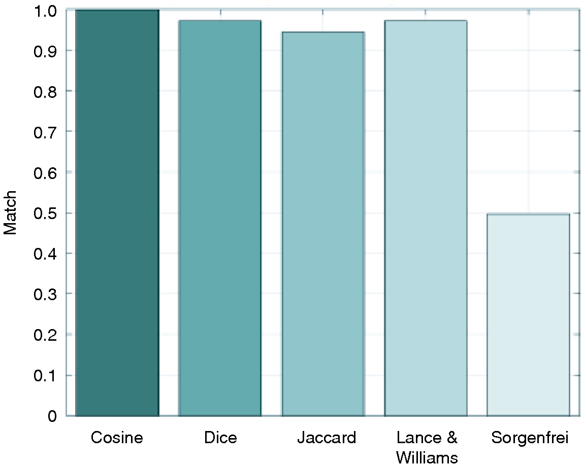
With respect to output (b), the existence of a particular modular structure, we repeat the analysis described in Section 4.3. For every additional similarity measure tested, we first generate an ensemble of 1000 networks. For each ensemble, we identify the module to which each risk is most frequently assigned, and compare this with its respective module assignment obtained using cosine distance. Figure 5 maps the overall match between the cluster assignment obtained using cosine distance and the additional similarity measures. In general, module assignment under Dice, Jaccard, and Lance and Williams similarity measures is almost identical to that obtained using cosine distance. This is not the case for Sorgenfrei, where the match is poor.
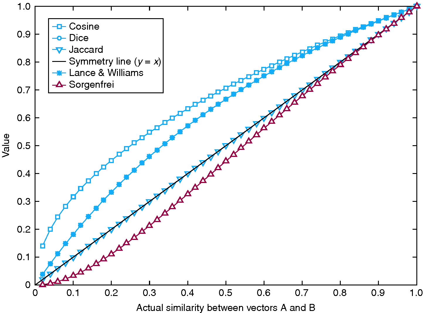


To identify the cause for this poor match, we performed a simple experiment to assess the sensitivity of each measure with respect to vector similarity. Consider vectors A and B, the first being composed of 0s and the latter of 1s. At this point, the similarity between A and B is 0. At each time step, vector A becomes incrementally similar to vector B by randomly choosing a 0 entry and switching its value to 1. Therefore, vector A becomes increasingly similar to vector B at every time step, until they become identical. At this point, the similarity between A and B is 1. By monitoring the increase in similarity using different similarity measures, we can assess the sensitivity of each measure. In this case, superlinear behavior corresponds to heightened sensitivity, while sublinear behavior corresponds to reduced sensitivity (see Figure 6). Evidently, measures that have a good match in terms of reporting the same modules – cosine, Dice, Jaccard and Lance and Williams (Figure 5, bars 1–3) – are those that grow at least linearly with increased similarity, while measures that grow sublinearly – Sorgenfrei (Figure 5, bar 4) – perform poorly.
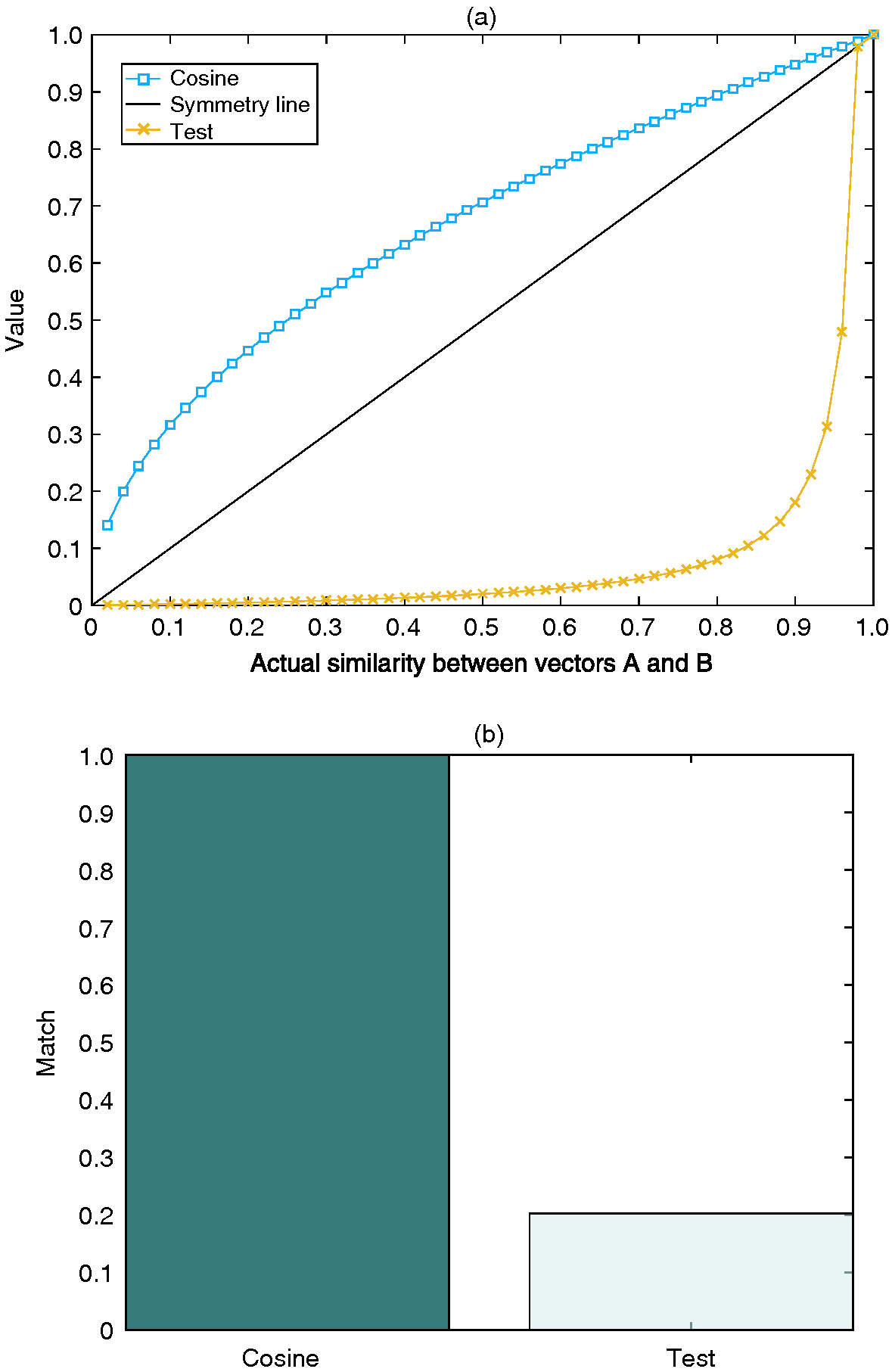
To assess the generalizability of this statement, we define an additional measure designed to grow minimally with increased similarity:
| (4.7) |
see Figure 7(a). As expected, the performance of this measure is exceedingly poor when considering the resulting cluster assignment in relation to those obtained using cosine distance (Figure 7(b)).
In conclusion, this section tests the dependency of the reported results with respect to the adopted similarity measure. The focus is on (a) the evident mismatch between independent and systemic risk impact, and (b) the particular modular structure that characterizes the risk network. Both (a) and (b) are robust against the use of similar similarity measures, as shown in Table 4 and Figure 5. However, the robustness of (b) has an additional caveat; the measures used to evaluate similarity grow at least linearly with respect to the number of shared characteristics (Figure 6). Considering the nature of the data examined herein, this is a reasonable expectation, as every additional positive match between two characteristic vectors contributes to the similarity of their respective risks.
Declaration of interest
This work was partly funded by ORIC International (C.E., N.A. and C.C.) and an EPSRC Doctoral Prize Fellowship (C.E.). C.E. and N.A. were partly, and C.C. fully, employed by ORIC International, a nonprofit organization in the (re)insurance and asset management sector, at the time of writing. The authors report no conflicts of interest. The authors alone are responsible for the content and writing of the paper. Note: the data set supporting the conclusions of this paper is included within the paper and its additional files, which are available online. This article is distributed under the terms of the Creative Commons Attribution 4.0 International License, https://creativecommons.org/licenses/by/4.0/.
Acknowledgements
We are grateful to Jenna Anders of ORIC International for useful comments, discussions and support. C.E. and N.A. designed the experiment; C.C. provided the data set; C.E. developed the model, analyzed the data, prepared figures and wrote the manuscript; and C.E., N.A. and C.C. reviewed and approved the manuscript.
References
Albert, R., and Barabási, A.-L. (2002). Statistical mechanics of complex networks. Reviews of Modern Physics 74(1), 47–97 (http://doi.org/cb5h4c).
Allan, N., Cantle, N., Godfrey, P., and Yin, Y. (2013). A review of the use of complex systems applied to risk appetite and emerging risks in ERM practice. British Actuarial Journal 18(01), 163–234 (http://doi.org/bwnf).
Arenas, A., Fernandez, A., and Gomez, S. (2008). Analysis of the structure of complex networks at different resolution levels. New Journal of Physics 10(5), 053039 (http://doi.org/fpffd9).
Basel Committee on Banking Supervision (2010). Basel III: a global regulatory framework for more resilient banks and banking systems. Report, Bank for International Settlements.
Battiston, S., Puliga, M., Kaushik, R., Tasca, P., and Caldarelli, G. (2012). Debtrank: too central to fail? Financial networks, the Fed and systemic risk. Scientific Reports 2, 541 (http://doi.org/gbbqvq).
Battiston, S., Caldarelli, G., D’Errico, M., and Gurciullo, S. (2016a). Leveraging the network: a stress-test framework based on DebtRank. Statistics and Risk Modeling 33(3–4), 117–138 (http://doi.org/bzz3).
Battiston, S., Farmer, J. D., Flache, A., Garlaschelli, D., Haldane, A. G., Heesterbeek, H., Hommes, C., Jaeger, C., May, R., and Scheffer, M. (2016b). Complexity theory and financial regulation. Science 351(6275), 818–819 (http://doi.org/cbtt).
Bearman, P. S., and Parigi, P. (2004). Cloning headless frogs and other important matters: conversation topics and network structure. Social Forces 83(2), 535–557 (http://doi.org/c64stw).
Bernstein, P. L. (1996). Against the Gods: The Remarkable Story of Risk. Wiley.
Besley, T., and Hennessy, P. (2009). The global financial crisis – why didn’t anybody notice? British Academy Review 14, 8–10.
Bidart, C., and Charbonneau, J. (2011). How to generate personal networks: issues and tools for a sociological perspective. Field Methods 23(3), 266–286 (http://doi.org/cfm8x9).
Blondel, V. D., Guillaume, J.-L., Lambiotte, R., and Lefebvre, E. (2008). Fast unfolding of communities in large networks. Journal of Statistical Mechanics: Theory and Experiment 2008(10), P10008 (http://doi.org/bxz74q).
Buchanan, L., and O’Connell, A. (2006). A brief history of decision making. Harvard Business Review 84(1), 32–41.
Choi, S.-S., Cha, S.-H., and Tappert, C. C. (2010). A survey of binary similarity and distance measures. Journal of Systemics, Cybernetics and Informatics 8(1), 43–48.
Clauset, A. (2005). Finding local community structure in networks. Physical Review E 72(2), 026132 (http://doi.org/frm4d3).
Danon, L., Diaz-Guilera, A., Duch, J., and Arenas, A. (2005). Comparing community structure identification. Journal of Statistical Mechanics: Theory and Experiment 2005(09), P09008 (http://doi.org/ctw6ht).
DasGupta, B., and Kaligounder, L. (2014). On global stability of financial networks. Journal of Complex Networks 2(3), 313–354 (http://doi.org/bhxs).
Fortunato, S. (2010). Community detection in graphs. Physics Reports 486(3), 75–174 (http://doi.org/b48x7f).
Fortunato, S., and Barthélemy, M. (2007). Resolution limit in community detection. Proceedings of the National Academy of Sciences 104(1), 36–41 (http://doi.org/fk9d9v).
Ganin, A. A., Massaro, E., Gutfraind, A., Steen, N., Keisler, J. M., Kott, A., Mangoubi, R., and Linkov, I. (2016). Operational resilience: concepts, design and analysis. Scientific Reports 6, 19540 (http://doi.org/f77hdx).
Girvan, M., and Newman, M. E. J. (2002). Community structure in social and biological networks. Proceedings of the National Academy of Sciences 99(12), 7821–7826 (http://doi.org/c85prm).
Gutfraind, A. (2010). Optimizing topological cascade resilience based on the structure of terrorist networks. PloS One 5(11), e13448 (http://doi.org/c43z3g).
Helbing, D. (2013). Globally networked risks and how to respond. Nature 497(7447), 51–59 (http://doi.org/f4vhxb).
International Actuarial Association (2008). Practice note on enterprise risk management for capital and solvency purposes in the insurance industry. Report, IAA, Ottawa.
International Organization for Standardization (2009). ISO 31000:2009 – risk management – principles and guidelines. Report, ISO, Geneva.
Kaplan, R. S., and Mikes, A. (2012). Managing risks: a new framework. Harvard Business Review 90(6), 49–60.
Kelliher, P., Wilmot, D., Vij, J., and Klumpes, P. (2013). A common risk classification system for the actuarial profession. British Actuarial Journal 18(01), 91–121 (http://doi.org/cbt5).
Lesot, M.-J., Rifqi, M., and Benhadda, H. (2008). Similarity measures for binary and numerical data: a survey. International Journal of Knowledge Engineering and Soft Data Paradigms 1(1), 63–84 (http://doi.org/cmg5dh).
Merluzzi, J., and Burt, R. S. (2013). How many names are enough? Identifying network effects with the least set of listed contacts. Social Networks 35(3), 331–337 (http://doi.org/f47tn4).
Newman, M. E. (2004). Analysis of weighted networks. Physical Review E 70(5), 056131 (http://doi.org/fxdwft).
Newman, M. E. (2006). Modularity and community structure in networks. Proceedings of the National Academy of Sciences 103(23), 8577–8582 (http://doi.org/d97nt5).
Newman, M. E., Barabasi, A.-L., and Watts, D. J. (2011). The Structure and Dynamics of Networks. Princeton University Press.
Nicolini, C., Bordier, C., and Bifone, A. (2017). Community detection in weighted brain connectivity networks beyond the resolution limit. Neuroimage 146, 28–39 (http://doi.org/f9vm9n).
ORIC International (2017). A Network Science Approach to Emerging Risk: Executive Summary. ORIC International, London. Available upon request.
Pastor-Satorras, R., Castellano, C., Van Mieghem, P., and Vespignani, A. (2015). Epidemic processes in complex networks. Reviews of Modern Physics 87(3), 925–979 (http://doi.org/f7px35).
Pritchard, C. L. (2014). Risk Management: Concepts and Guidance. CRC Press.
Roukny, T., Bersini, H., Pirotte, H., Caldarelli, G., and Battiston, S. (2013). Default cascades in complex networks: topology and systemic risk. Scientific Reports 3, 2759 (http://doi.org/cbt6).
Schweitzer, F., Fagiolo, G., Sornette, D., Vega-Redondo, F., and White, D. R. (2009). Economic networks: what do we know and what do we need to know? Advances in Complex Systems 12(04n05), 407–422 (http://doi.org/ccbc5k).
Sneath, P. H., and Sokal, R. R. (1973). Numerical Taxonomy: The Principles and Practice of Numerical Classification. W. H. Freeman.
Squartini, T., and Garlaschelli, D. (2011). Analytical maximum-likelihood method to detect patterns in real networks. New Journal of Physics 13(8), 083001 (http://doi.org/bkbjtw).
Szymanski, B. K., Lin, X., Asztalos, A., and Sreenivasan, S. (2015). Failure dynamics of the global risk network. Scientific Reports 5, 10998 (http://doi.org/cbt7).
Vespignani, A. (2012). Modelling dynamical processes in complex socio-technical systems. Nature Physics 8(1), 32–39 (http://doi.org/fzkmbs).
Watts, D. J. (2002). A simple model of global cascades on random networks. Proceedings of the National Academy of Sciences 99(9), 5766–5771 (http://doi.org/fh2khd).
World Economic Forum (2017). The global risks report 2017. Report, January 11, WEF.
Only users who have a paid subscription or are part of a corporate subscription are able to print or copy content.
To access these options, along with all other subscription benefits, please contact info@risk.net or view our subscription options here: http://subscriptions.risk.net/subscribe
You are currently unable to print this content. Please contact info@risk.net to find out more.
You are currently unable to copy this content. Please contact info@risk.net to find out more.
Copyright Infopro Digital Limited. All rights reserved.
As outlined in our terms and conditions, https://www.infopro-digital.com/terms-and-conditions/subscriptions/ (point 2.4), printing is limited to a single copy.
If you would like to purchase additional rights please email info@risk.net
Copyright Infopro Digital Limited. All rights reserved.
You may share this content using our article tools. As outlined in our terms and conditions, https://www.infopro-digital.com/terms-and-conditions/subscriptions/ (clause 2.4), an Authorised User may only make one copy of the materials for their own personal use. You must also comply with the restrictions in clause 2.5.
If you would like to purchase additional rights please email info@risk.net
